
Intro to running Python
IPython, now known as Jupyter, is a REPL based system that allows you to embed code into a web-based document containing other information: text, images, data, etc. This is an incredibly powerful advance: it not only allows you to audit your code, describing it in detail and distributing it with the associated data and visualizations, but it allows you to build code into documents such that you can connect to data in the real world and re-run the code, keeping the document continually up to date. Increasingly, scientific journals are accepting Jupyter Notebooks as online paper appendices.
Not only do the Notebooks provide REPL areas within a document, but they provide enhancements to the REPL environment, and a wide variety of save options – including saving the documents as stand-alone webpages that work without Jupyter and PDFs.
IPython Notebooks were, as the name suggests, initially a Python REPL project. However, the project has expanded to allow other REPL languages, for example R, to be integrated, and therefore has been renamed to Jupyter Notebooks. You can find out more about setting up other languages by looking at "kernels" in the Jupyter documentation. Despite the overall project name changing, people talk about iPython Notebooks as the kernel (~language interpreter) for Python is still called iPython. Note also that, as we've seen, the iPython interpreter is built into other software, so Spyder uses it as its default console, for example.
You can download Jupyter Notebooks separately from the Jupyter project website, but it also comes bundled with Anaconda. Let's open it now.
To open Jupyter, type the following at the command prompt/terminal:
jupyter notebook
You should find a web browser opens showing the current directory, and all the directories within it. You can navigate to other directories in the starting one if you aren't happy with where you are (one minor issues (probably the only one) is that it is hard to navigate to other parts of the file system to open other Notebooks if the directories aren't where you started, so always start low down the directory structure).
Find the New drop down list at the top of the page, and choose Python 3 This will open up a Notebook and intermittently save it to the current directory (although it does save now and then, it's good practice to save your workbook as you go along using the disk icon to be sure).
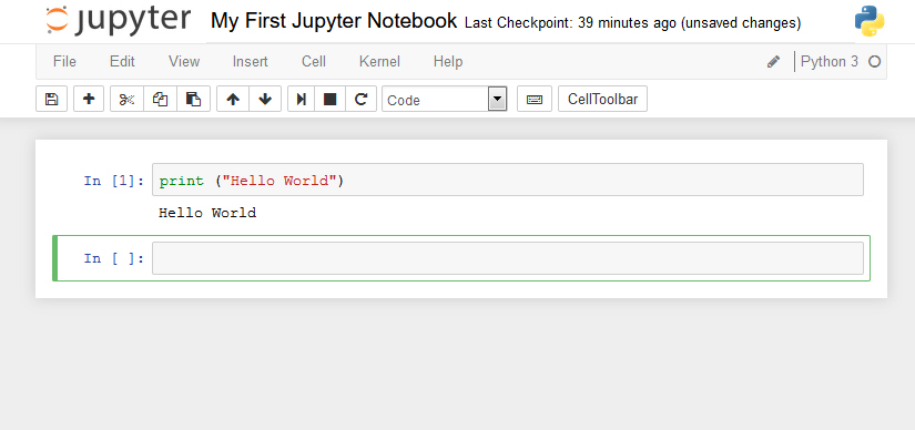
You'll see that at the top of the page, there's a title, set by default to "Untitled". Click this and change it to My First Jupyter Notebook or similar. This title will be used as the filename for the notebook. Notebooks have the file extension .ipynb, so if you restart Jupyter and need to reopen the notebook, look for the My First Jupyter Notebook.ipynb file.
You'll see that the webpage starts with a box to type in. Type the "Hello World" program into this box, then press SHIFT and ENTER together. This will run the program.
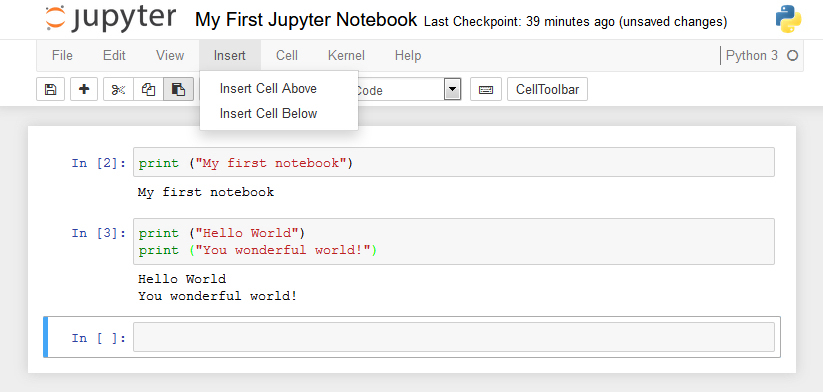
You can type a set of lines (indeed, a whole program) into one box, going back and adding extra lines to a pre-existing box. Note that if you need to indent (you don't for this program) the TAB key indents multiple selected lines, and the SHIFT + TAB key together remove one level of indenting.
You can use the insert menu to add new boxes above or below the current one, and the Edit to remove the currently selected cell.
If you need to rerun the code in a box (because it has an error or because you want to refresh the results) just click in it and SHIFT ENTER.
If you have multiple boxes, and they rely on each other, you only have to re-run those that are lower down after you change something – the results of the boxes above don't need re-running.
As for what goes in the boxes, these are usually two things: either Python code, or a simple text formating language called "Markdown".
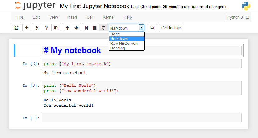
To see some markdown, make a fresh box and click in it. Go to the dropdown menu that says Code and change it to Markdown and then type the following markdown in an empty box:
# My notebook
SHIFT ENTER to translate/compile it from markdown to HTML, the language displayed in webpages.
You'll see it appears as a header. To re-edit the markdown, double click the new text.
There's a cheat sheet for markdown here.
The iPython kernel specifically also enhanses the Python REPL options with "magic" functions (these may or may not be implemented in other Jupyter languages). These start with one or two percentage signs, so, for
example %reset clears all the variable values. There is a full list
on the Python website, but other useful commands include
%reset_selective; %run; %save; %sx (run something on the underlying operating system; %timeit (for timing how long a
set of lines takes to run). You can also use magic commands to run cells using other languages – see the bottom of the
documentation for details.
One specifically useful set of magic commands are those replicating the standard Linux commands to naviage directories. This helps, for example, with reading and writing data files. These generally work without the percentage signs, so:
pwd – tells you your present working directory (i.e. which directory you are in).
cd somename – moves you to the directory called somename within the current directory.
cd .. – moves you to the directory containing the directory you are in.
cd ~ – takes you to your home/user directory.
So, for example, say pwd tells us we are in our temp directory, and we want to get to a data directory on our Desktop, the following will get us there us:
cd ~/Desktop
cd data
If we then want to move to the Desktop directory, we could type:
cd ..
Have a go at moving around, using pwd to keep track of where you are.
Finally, to turn Jupyter off, close the webpages and then the command line. To kill Jupyter off (for example if it hangs), close the webpages and at the command line, press CTRL + c together (you may have to do it twice). CTRL + c generally kills things off at the command line. If you want to save the page as a static webpage to use in displaying the code, or a PDF, those options are under File -> Download (the PDF option needs a piece of software called LaTex installing).
Jupyter is a very powerful system, and we've only touched on its capabilities here. There's lots more to explore in the Notebooks, but for the moment, here's an example of it's capabilities: Example_Notebook.ipynb. Right-click the link and save the file somewhere, then navigate to the directory, open Jupyter Notebook, and the open the file. Run the only code cell in there to show how you can build interactivity into notebooks. You're not expected to understand the code at this stage, but if you can an inkling of how it works, all the better.
Once you've done that, we're done for this practical. Hopefully you have a pretty conprehensive overview of how Python is run (with the exception of running it inside other applications like ArcGIS or QGIS). We've seen:
- how to run a file you've developed or been sent using the command line;
- how to use the Python shell in a REPL fashion;
- how to use REPL and scripts together in IDLE;
- a more sophisticated IDE, in the form of Spyder;
- and, finally, an exciting REPL environment in the form of Jupyter Notebooks.