GEOG5870/1M: Web-based GIS A course on web-based mapping
Adding overlays
Markers are an example of one sort of overlay that can be placed on top of the background map in Google Maps. As we have seen earlier, it is possible to alter the marker image; one implication of this is that different marker styles can be used to convey additional information about the location (e.g. markers of different colours could be used to show different types of location). There are a variety of alternative overlays that can also be used in Google Maps, and we will look at some of these now.
Creating and adding lines and polygons
The Blue Plaques practical task, and most of the examples that we studied earlier focused on using markers to represent information. These are ideal for point level information, but not so good for area level information. An obvious thing to want to do is to draw lines and polygons on the map. The sample code shown below is for a map which will be drawn with a set of overlay lines. Three files are illustrated.
The first of these is the HTML file which will contain our map. The HEAD section contains links to a number of other files:
- The Google Maps JavaScript API
- The JSCoord library used in the previous module
- A JavaScript data file
- A JavaScript map setup file
- A JavaScript js file
- A JavaScript file called: commonmaputilpoly.js which contains additional methods for constructing polygons and lines.
- Two style sheets a general one (intended for general page appearance) and a more map specific one
The code for lines.html
<!DOCTYPE html>

<html>

<head>

 <script type="text/javascript"

   src="http://maps.google.com/maps/api/js"></script>

 <script type="text/javascript" src="jscoord-1.1.1.js"></script>

 <script type="text/javascript" src="linesdata.js"></script>

 <script type="text/javascript" src="lines.js"></script>

    type="text/css">

 <title>Google Maps examples - lines</title>

</head>


<body onload="initialize()">


<h1>Google Maps examples - lines</h1>


<p>[ <a href="../index.html">Personal home page</a>

   | <a href="index.html">Geog5870 work</a> ]</p>

  <div class="gmap" id="map_canvas" style="height: 800px; width: 600px">

     </div>

<p>This maps shows migration flows from districts

   of the UK to Leeds, as recorded in the 2001 Census.</p>

<ul>

<li>Source: 2001 Census: Special Migration Statistics

<li>Census output is Crown copyright and is reproduced

   with the permission of the Controller of HMSO

   and the Queen's Printer for Scotland.

</ul>

  </body>

</html>
The body of the HTML is much the same as in previous examples, although as
we will be drawing a map of the UK in this example, I have made the map_canvas
DIV long and thin.
The second file shown is an excerpt of a data file, showing the general structure. This was converted from CSV exported from an Excel spreadsheet; all values have been placed in quotes. The data are taken from the 2001 Census Special Migration Statistics, and detail migration flows from different districts of the UK to Leeds. The 'origin' value is simply a district number, and the 'flow' value is the number of persons recorded in the Census who had changed their usual residential address in the year prior to the Census. For each data value, the flow shows the number of people who lived in Leeds at the time of the Census, and in the origin district one year before the Census.
The full file can be downloaded here.
The code for linesdata.js
var os_flows = [{

   "origin":"1",

   "easting":"532482.0205",

   "northing":"181269.0031",

   "flow":"3"

	},

	{

   "origin":"2",

   "easting":"548069.5347",

   "northing":"185093.88",

   "flow":"7"

	},

	{

   "origin":"3",

   "easting":"524027.288",

   "northing":"192316.1974",

   "flow":"182"

	},

	{

   "origin":"4",

   "easting":"548802.2259",

   "northing":"175489.3452",

   "flow":"30"

	},
The third file shown is the map set up file. This sets up a map in the same way as done in the previous examples. It then iterates through a data set, again as in previous examples with markers. However, in this case we are doing something different with the data: we are drawing lines on the map.
The code for lines.js
var map; // The map object

var myCentreLat = 53.825740;

var myCentreLng = -1.506015;

var initialZoom = 6;


function initialize() {

   /*

    * In this example, lines are from each origin

    * to a known destination point which is also

    * the map centre

   */

   var myDest = new google.maps.LatLng(myCentreLat,myCentreLng);


   var myOptions = {

      zoom: initialZoom,

      center: myDest,

      mapTypeId: google.maps.MapTypeId.ROADMAP

   };


   map = new google.maps.Map(

      document.getElementById("map_canvas"),myOptions);


   var info = "";


   for (id in os_flows) {


      // Convert co-ords

      var osPt = new OSRef(os_flows[id].easting,os_flows[id].northing);

      var llPt = osPt.toLatLng(osPt);

      llPt.OSGB36ToWGS84();

      var myOrig = new google.maps.LatLng(llPt.lat,llPt.lng);


      /*

       * Construct a flow line

       *

       * In this example, lines are from each origin

       * to a known destination point

       * Destination is hard coded here for sake of simplifying code

      */

      var flowLine = new google.maps.Polyline({

         path: [myOrig,myDest],

         strokeColor: "#FF0000",

         strokeOpacity: 1.0,

         strokeWeight: 2

      });

      flowLine.setMap(map);


   }


}
Here's what this should look like as standard:
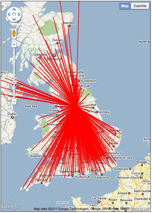
The lines that have been added are called polylines in the Google
Maps API. Polyline is defined by a series of points; this map uses the simplest
of such lines, which are defined by only a start and an end point. Let us
return to the code shown in the map setup script above. The loop
'for (id in os_flows) {}' iterates through the data array, carrying
out its body section once for each data point.
The first task within this loop – as with the
Blue Plaques example – is to convert the location data from OS
grid references to lat-lng data points. In this example, we construct a LatLng
object called myOrig from each point we read. Note that despite
the fact that the eastings and northings are quoted in the data file, and might
thus be thought of as strings, the LatLng constructor is happy to treat them as
numeric values.
Next in the loop we draw the line. There are two stages to this. Firstly, we construct
a polyline object, using 'new google.maps.Polyline()'. This
requires one parameter – an object which lists line co-ordinates and the various
options.
      var flowLine = new google.maps.Polyline({

         path: [myOrig,myDest],

         strokeColor: "#FF0000",

         strokeOpacity: 1.0,

         strokeWeight: 2

      });
The most important of these are the line co-ordinates. These are given
in the path property of the polyline parameters object. The path is
an array, containing a set of points, each of which is a
google.maps.LatLng() object. We use two points: the
myOrig point that has just been created (as converted from the OS
grid references), and a second point myDest. As this map shows
flows to one location only we define the destination once (at the top of the file), and use the same
point each time in our path.
The other characteristics for a polyline are the colour, opacity and width of the line. In this initial example, we have drawn all lines with the same characteristics: opaque red lines of weight 2.
The final thing that we need to do is add the line that has now been defined to the map. The is done in the statement:
flowLine.setMap(map);
We use the setmap() method
of the generic google.maps.Polyline() object to attach the line to
the map, giving the name of the map object to which we wish to attach the line.
As you can see from the code above, the resulting map contains a mass of lines, which does not tell us much apart from the fact that – like most large cities, especially those with large universities, Leeds draws migrants from almost everywhere in the country. Ideally we need to make the lines clearer and more meaningful.
Improving the lines
We can alter the setup program to change the line style for flows of
different size. The following code shows excerpts from the code of a revised example.
Some changes have been made within the initialize() function.
Firstly, we have added three new variables, myColor,
myOpacity and myWeight; as we intend to alter these
characteristics for each line.
We have also added a set of statements into the for loop that cycles through
each data point. We have a series of if {} statements, which set
up the line characteristics. These are structured so that large flows which
meet all the 'if' criteria (i.e. they're greater than 0, they're also greater
than 10 etc...) will over-write the previous values for myColor
etc.
Excerpts from lines2.js
  var myColor;

  var myOpacity;

  var myColor;


  for (id in os_flows) {


   //...


   if (os_flows[id].flow > 0) {

      myColor = "#000000";

      myOpacity = 0.2;

      myWeight = 1;

   }

   if (os_flows[id].flow > 10) {

      myColor = "#000000";

      myOpacity = 0.3;

      myWeight = 1;

   }

   if (os_flows[id].flow > 100) {

      myColor = "#EE0000";

      myOpacity = 0.7;

      myWeight = 2;

   }

   if (os_flows[id].flow > 1000) {

      myColor = "#EE0000";

      myOpacity = 0.9;

      myWeight = 3;

   }


   var flowLine = new google.maps.Polyline({

      path: [myOrig,myDest],

      strokeColor: myColor,

      strokeOpacity: myOpacity,

      strokeWeight: myWeight

   });

   flowLine.setMap(map);

}
The lines are set to be drawn in black (but thin, and fairly transparent) if the flow is small, and in red (and thicker, and more opaque) if the flow is larger. This stage is clearly in the arena of basic map design – one needs to know something about the nature of the data being mapped and about the range of possible values, and then try out various different line styles.
Here's a file to run this; it looks like this:
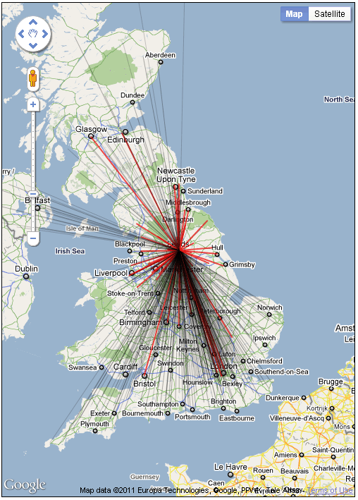
The map is clearer, and it is possible to distinguish those origins from which the major flows are drawn, although it is still quite crowded – a common result in maps of this type. Further improvements might be made with changes to the line styles, and we might also decide to only draw those lines that represent flows above a certain threshold (say, 50 persons).
As with any map, the framing page should give some sort of explanatory key when lines are shown in different colours to convey some quantitative meaning.
As described above, a polyline is a line made up of a number of segments (in the above example, only one segment per line) defined as a set of co-ordinates. The step from this to a polygon is straightforward: a polygon is a line which returns to its initial starting point. Polygons have the additional characteristic beyond a line in that they can have a fill colour (and variable fill opacity) as well as line characteristics.
The following listing shows the code of a set of files which illustrate the construction
of basic polygons. The structure of these files is similar to those that we
used before, but we will run through their contents.
The HTML file poly1.html is illustrated first. It is very similar to the file used in the line drawing above, differing only in the names of the files loaded, and the on-page text.
The HTML file poly_eg1.html
<!DOCTYPE HTML>

<html>

<head>

<meta http-equiv="content-type" content="text/html; charset=ISO-8859-1">

 <script type="text/javascript"

 src="http://maps.google.com/maps/api/js"></script>

 <script type="text/javascript" src="jscoord-1.1.1.js"></script>

 <script type="text/javascript" src="poly_eg1_data.js"></script>

 <script type="text/javascript" src="poly_eg1_setup.js"></script>


 <title>Google Maps examples - polygons</title>


</head>


<body onload="initialize()">


<h1>Google Maps examples - polygons</h1>

<p>[<a href="../index.html">Personal home page</a>

| <a href="index.html">Geog5870/1 examples</A>]</p>

   <div class="gmap" id="map_canvas" style="height: 300px; width: 400px;">


<p>This example looks at the process of adding a polygon</p>

</body>

</html>
The second file is a data file. It defines two polygons with some basic
details, and a boundary property which contains an array of grid
reference points.
The data file poly_eg1_data.js
/*

 * A set of data which will be used to draw polygons

 */

var os_polydata = [{

   'title': 'poly1',

   'description': 'poly1',

   'value': "7",

   'boundary': [

      {'easting':430000,'northing': 433000},

      {'easting':430000,'northing': 434000},

      {'easting':431000,'northing': 434000},

      {'easting':431000,'northing': 433000}]

   },

   {

   'title': 'poly2',

   'description': 'poly2',

   'value': "88",

   'boundary': [

      {'easting':428000,'northing': 433000},

      {'easting':428000,'northing': 434000},

      {'easting':429000,'northing': 434000},

      {'easting':429000,'northing': 433000}

   ]
}];
The final file illustrated above is poly_eg1.js. Again, it is broadly similar to the previous examples. Instead of drawing lines or creating markers, the main loop in the initialize() function will create some polygons.
The data file poly_eg1_setup.js
var map; // The map object

var myCentreLat = 53.81;

var myCentreLng = -1.52;

var initialZoom = 12;


function initialize() {


   var myCentre = new google.maps.LatLng(myCentreLat,myCentreLng);


   var myOptions = {

      zoom: initialZoom,

      center: myCentre,

      mapTypeId: google.maps.MapTypeId.ROADMAP

   };


   map = new

      google.maps.Map(document.getElementById("map_canvas"),myOptions);


   for (id in os_polydata) {


      var polyPath = []; // An empty array


      /*

       * Read through points

      */

      var thisBoundary = os_polydata[id].boundary;


      for (pt in thisBoundary) {

         var osPt =

            new OSRef(thisBoundary[pt].easting,
            thisBoundary[pt].northing);

         var llPt = osPt.toLatLng(osPt);

         llPt.OSGB36ToWGS84();

         var myLatLng = new google.maps.LatLng(llPt.lat,llPt.lng);

         polyPath.push(myLatLng);

      }


      /*

       * Construct the polygon

      */

      myPoly = new google.maps.Polygon({

         paths: polyPath,

         strokeColor: "#FF0000",

         strokeOpacity: 0.8,

         strokeWeight: 3,

         fillColor: "#FF0000",

         fillOpacity: 0.35

      });


      myPoly.setMap(map);

   }

}
- We create the variable
polyPathas an empty array. This will contain thepaththat defines the polygon. - We copy the
boundaryproperty of the current object being read from the data array (we could work directly onos_polydata[id].boundarybut this is simplier to read). - We start a new loop (nested inside the main loop that is processing the data file) to read through the boundary object.
- For each point, we follow the previously illustrated process of conversion from OS grid reference to WGS84 Latlng.
- We add the new point to our path. This is done using
polyPath.push(point).push()is a method attached to the genericArrayobject, and it adds the argument (in our case, a point) to the end of the array. - Having finished processing all of the boundary points, we construct a new
google.maps.Polygon()object. This takes a number of parameters. The stroke parameters refer to the boundary line, whilst the fill parameters refer to the middle of the polygon. - We add the polygon to the map using the
setmap()method of the Polygon object (in the same way as we did with the lines).
Here's what it should look like:
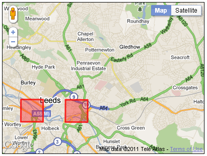
It can be seen that the polygons are simple squares, with a solid red outline and semi-opaque fill.
Summary
On this page, we have seen examples of how we can add lines and polygons to
a map. The lines example showed how a reasonably large number of lines can be
added, whilst the polygon example used a simpler case. In the case of polygons,
we can generate complex polygons as well as these very simple examples – you
may note that the boundary data was added to the polygon property
paths rather than path as was the case with the
polyline. With polygons, we can add multiple paths, and thus have polygon
objects with more than one component; we can also define polygons with 'holes'
in them.
On the next page , we shall look at how we can add information to polygons.
[ Next: Adding information to polygons ]