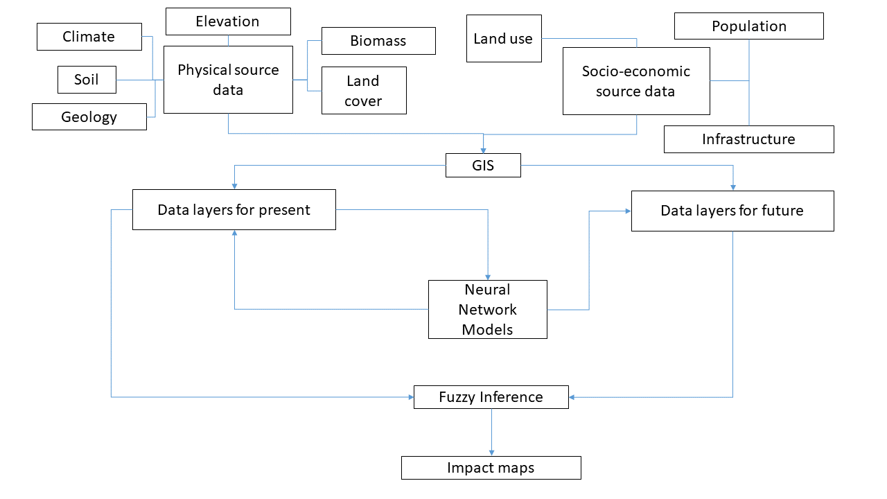
Figure 1. The basic Synoptic Prediction System model
Stan Openshaw, Tim Perrée, Andy Turner, and Ian Turton
Contents
The principal objective of Project 9.1 was to integrate socio-economic dimensions of land degradation with on going MEDALUS III environmental modelling activities. This involved developing a means of modelling the linkages between physical, climatic and socio-economic change using a GIS-based approach. The methodology and computer models developed to meet this objective are far more complex and sophisticated than was originally anticipated as it became apparent that considerable research innovation was required to achieve any major scientific results. The three initial aims in 1996 were:
By mid-way through the project it was evident that the only feasible realistic way to estimate socio-economic impacts was to re-interpret what was regarded as a socio-economic impact. It was clearly impossible to produce 1 km2 estimates of climate related EU crop subsidy changes for durum wheat for 2050 (or even 1998) or to model the detailed spatial impact of climate change on unemployment levels or migration rates or age-sex profiles. Instead it is argued that the best broad spectrum indicator of overall socio-economic effects in the Mediterranean climate region of the EU is land use change and particularly that related to land degradation itself. In rural economies land quality is what matters and it is this aspect of the environment most at risk from climate change. The objective was to develop an integrated computer model able to link climatic and physical environmental change with likely socio-economic trends to predict land use change at a fine geographical scale. Termed the Synoptic Prediction System (SPS) this has been designed to operate at a level of geographic resolution equivalent to the existing climatic and other environmental process data available to Medalus project teams. Considerable effort has been expended in designing creating and developing the SPS model based on a hybrid of artificial neural networks and advanced fuzzy logic methodologies. The result is a mark 1 prototype integrated climatic, environmental, and socio-economic modelling system capable of making plausible scenario based predictions of possible environmental impacts on land use and land degradation for about 40 to 80 years ahead. The SPS is the first of its kind and its development is arguably a most significant scientific achievement. Other useful outputs from this project include the 1-decimal-minute resolution geographical database for the entire Medalus Mediterranean study region. This is comprised of climatic, physical and socio-economic data in a common spatial framework at an identical geographical scale. Maps of these data can be viewed from an extensive set of web pages which have been created to document Project 9.1, disseminate the results and data products and promote an interactive GIS style interface to these data; see the following URL for details: http://www.medalus.leeds.ac.uk/SEM/home.htm
This final report is a summary of those web pages.
There is a growing likelihood that global climatic change will start to have a visible and increasingly fundamental environmental and socio-economic impact in the next half a century over many parts of the world. In some regions, such as Northern Europe, the effects may well be unnoticed or are irrelevant because they are well within the capacity of existing ecosystems to cope or are economically irrelevant; however, in other regions including the Mediterranean climate region of the EU the environment is far more fragile and climate change gives justifiable cause for concern. Indeed in most of the Mediterranean climate regions (including those in non-EU countries) it is possible that even small changes in climate will be sufficient to cause a major detrimental local and regional impacts on the physical environment and related socio-economic systems. The research challenge for this project has been to develop a plausible way of making reasonable predictions of the effect of climatic change on socio-economic systems for about 50 or more years hence and then use this as a basis for raising awareness and creating a framework for action. Note that here the term socio-economic systems has been interpreted in an indirect and aggregate fashion by trying to identify their integrated effects on patterns of rural land use. This is considered more useful and relevant to Medalus than focusing on employment opportunities, demographic change or other specific socio-economic factors which although related to land degradation are connected and influenced by political and economic systems that are extremely hard to model with current technology and impossible to forecast accurately in a highly detailed spatial way.
The complexity of this scientific challenge addressed by Project 9.1 should not be underestimated. Yet there is an increasing urgency to know something of what may be happening to our world in the medium term future so that strategic planning may be proactive rather than purely reactive. There really do have to be forecasts of the possible impacts of climate change for about 50 years hence if there is to be any hope of a significant and meaningful policy response by EU decision-makers. It is also important that a view of the whole picture is offered whereby the otherwise obscure physical and environmental impacts are translated and presented in a form that is readily understandable by non-geographers. Socio-economic factors influence land degradation far more than any change in the size distribution or moisture content of soil particles in a semi-arid zone but the processes are ill-defined, undeniably complex, non-deterministic, and probably chaotic. Yet ultimately the effect on people matters more than changes in base sediment load in a particular river system. Estimated changes in climatic biomass potential could conceivably be used to make people more aware of the problem. Yet although such individual physical measurements are "signs" of change and provide legitimate cause for concern, their meaning is probably too abstract to attract the necessary levels of public and political attention. The purely physical model results are mainly destined for science journals and are aimed at academics rather than the public and EU policy makers. Yet it is vital that the integrated effects of physical, climatic and socio-economic change can be translated in a way that is more readily and widely understandable. The research reported here is important because it attempts to model both physical and human systems in an integrated way at the finest feasible level of geographic scale using the best available science. Hopefully the results in terms of land use change and land degradation impacts that can be more readily interpreted and understood by those actors who can make a difference. In presenting the results we aim to retain the uncertainties in our predictions and have tried to be honest about the imperfections in what we have attempted. The challenge for others is to try and extend, improve and build on these efforts.
From a methodological perspective there has been very little research performed on predicting future land use patterns on a local let alone national or EU scale. Most computer models that exist are generally concerned only with very limited aspects of the problem; for instance, regional employment change or population dynamics or very short-term econometric modelling at a micro-scale. An exception is the work by the CLUE Group; see de Koning et al. (1997), Veldkamp and Fresco (1996, 1997), Verburg et al. (1997). The CLUE modelling framework (The Conversion of Land Use and its Effects) is based on a multi-scale stepwise linear regression model that attempts to express land use and land use change as a function of socio-economic and biophysical factors at an aggregate spatial scale for China, Ecuador, and Costa Rica. The model is a linear continuous time simulation at a fairly coarse spatial scale; ranging from 7.5 km2 for Costa Rica to 32 km2 for China. In our opinion, the EU requires something rather more sophisticated, the basic design requirements are:
So the seemingly limited initial objective of adding a socio-economic component to Medalus III was translated into the task of developing and applying a Synoptic Prediction System designed to estimate plausible impacts of global climatic change on land use patterns across the Mediterranean climate region of the EU. Designing and developing the system has been challenging because many of the theoretically desirable data sets are either not available or do not exist whilst there are significant uncertainties in all the data that do exist. Additionally, system process knowledge is woefully deficient as virtually all the principal mechanisms for linking the dynamics of the physical environment and climate with the associated socio-economic systems are as yet very poorly understood. In essence the underlying and most basic problem is that physical and climatic process models are far better developed than any of the models of socio-economic systems particularly those concerned with agricultural land use. If you ask the question `What is the likely effect of climatic change on the hydrology of a specific river catchment or on the speed of erosion of a particular hill slope?' - then methods exist that may indicate broad answers. If you ask the question `What is the likely impact of EU agricultural subsidies on the crops growing in the fields on this hill slope or on the agriculture of this catchment?' - then there are no existing models for the current situation let alone models which can predict the effect in 50 to 100 years time! Some kind of novel computer modelling methodology had to be devised to satisfy the forecasting objective, cope with the deficiencies in the available data, and manage without good process knowledge.
Our view is that presently a synoptic modelling system which implements a broad-brush GIS style of approach to the problem is the best available and probably the only feasible scientific option available today capable of making localised geographical predictions of the possible impacts of global climatic change on land use for up to 100 years time. This report describes the construction, application and development of a Synoptic Prediction System (SPS) that employs a mix of GIS, neurocomputing, and fuzzy logic technologies to attempt this almost impossible but potentially extremely important task.
The objectives were to:
The structure of the basic system is outlined in Figure 1. The simplest view is that of a series of key input variables that are related via a computer (neural network based) model to some outputs. This can be considered as a form of complex non-linear and non-parametric regression model where the mapping of the inputs onto the outputs employs a neurocomputing approach as the non-linear relationships are both little understood and are too ill defined for more conventional statistical or mathematical modelling specifications to work well. Table 1 briefly outlines some of the strengths and weaknesses of models based on artificial neural networks; see also Openshaw and Openshaw (1997). However, the SPS is not entirely neural network based. Indeed another major innovation is that at various appropriate stages fuzzy logic based inference is employed to translate the artificial neural network's predictions into crisp impacts by making use of relevant knowledge and other data.
In operationalising the SPS shown in Figure 1. the choice of input variables had to be restricted to those which could be generated from the data available for Medalus III research. The available variables are not ideal but then probably no one knows what would be ideal in this context.
There are various inadequacies associated with the modelling structure displayed in Figure 1. One problem is that the relationship between the climate, the physical environment, socio-economic factors, land use and land degradation is mediated and affected by at least the following: available technology, market mechanisms, historical tradition, inertia, culture, and various economic factors such as subsidies which have not been taken fully into consideration. All these aspects are currently invisible to the model and are not directly present in any of the available data; although their integrated effects are somewhat present in the current patterns of land use that the neural net model is being asked to represent. It would of course be nice to have a model into which the price of crops, EU agricultural subsidies, irrigation practices, and each farmer's micro-behaviour could be input and then make the model operate at a fine spatial scale for the entire EU. However, such a model is presently beyond technological feasibility and data availability. It is possible that such models could be built one day by discovering how to model individual people in artificial world laboratories using a bottom-up approach, but this is probably at least 10 to 20 years off. To address the research now we have been forced by scientific circumstances, data restrictions and ignorance to adopt more of an aggregate top down approach. Although it is hoped that the missing variables are invisibly present in the data that are used and are thus taken into account implicitly by the neural nets that are applied to model the relationships. This is probably a most optimistic view particularly when the forecasts made for 40-80 years hence assume a continuation, at the same level as today, of all these invisible influences which may or may not be having a direct impact. Unfortunately, there has been little choice in this matter given the urgency of the task and the constraints of current technology, knowledge, data, and research resources. However, in defence we would note that there need be no direct relationship between overall model performance and the accuracy of the individual model sub-components and the various data layers. Indeed one of the most compelling justifications for a fuzzy approach is the belief that there can come a point in conventional models where improved precision and more detail in the systems of equations can result in a deterioration of performance; see Kosko (1994).
The system outlined in Figure 1 involves the following steps:
There were major practical difficulties in assembling every data set needed for this project; see Table 2 and Table 3. The problems can be classified as:
Major differences exist in quality, scale, and aggregation between existing physical environmental-climatic and socio-economic data presenting a serious obstacle to straightforward integrated land use modelling. Physical models of land degradation generally operate at a much more detailed spatial and temporal scale compared to existing socio-economic models. Additionally, socio-economic data generally relates to irregularly shaped zones that are historically unstable and subject to continuous change, whereas physical environmental-climatic models tend to use and produce data in regular gridded structures albeit at a range of different scales. In fact a major reason that much of the environmental change research has ignored socio-economic systems is the lack of socio-economic data with an appropriate level of spatial and temporal detail so that they can be directly linked to the outputs from the environmental models; see Clark and Rhind (1991). This can be regarded as a most unfortunate and a very fundamental obstacle to all research in this very important area.
Most of the available environmental data for the EU was acquired and manipulated into a regular grid orientated at a spatial resolution of approximately 1 km2 using GIS. A grid was selected as the spatial framework in which to store, manipulate, link and map the data since it offers the greatest flexibility in aggregating upwards and can yet still provide a realistic representation of regional or local variation provided the grid cells are sufficiently small in size. A geographical latitude-longitude projection was chosen as a compromise given the traditional problems in map projections regarding the representation of distance, direction and area distortion of the data caused by the curvature of the earth. A 1-decimal-minute (1 DM) resolution which is roughly equivalent to a 1 km2 scale for most of the EU was selected as providing the most appropriate and probably the best possible level of spatial resolution that was practicable for this research.
A common spatial framework for all the available climatic, environmental, and socio-economic data was an essential pre-requisite before any integrated modelling could be attempted. Aggregation upwards is fairly trivial but interpolation from coarse to finer levels of spatial resolution is far more problematic and error prone yet this is an unavoidably essential activity that needed to be mastered before much progress could be made. Virtually every data source involved in the SPS had a unique set of problems associated with it and necessitated various GIS operations and sometimes modelling applications to create a common scale database. In so doing various novel geo-processing methods were invented to handle problems associated with the aggregation and disaggregation of spatial data grids.
The first data set to be processed was the Global Land 1 km Base Elevation source data (GLOBE); see Eidenshink and Faudeen (1996). This 30 arc-second (or 0.5 DM) resolution grid in a geographical latitude-longitude projection was imported into ArcInfo and aggregated to a resolution of 1 DM as follows. Firstly, the 0.5 DM grid was aggregated from each of the four corners of the origin cell of that grid to produce four 1 DM resolution grids where the value in each 1 DM cell was assigned the mean value of the four 0.5 DM cells from which it was composed. These four 1 DM resolution grids were then disaggregated back to the 0.5 DM resolution where each cell was assigned a quarter of the average value at the 1 DM resolution. Now spatial consistent, the four disaggregated grids at a 0.5 DM resolution were combined to produce a single 0.5 DM grid where each cell was assigned the average of the four incident grid values. Finally, these averaged measurements were then aggregated back to a 1 DM resolution (selecting the correct point of aggregation so as the aggregate data fit the chosen common spatial framework) where again each cell was assigned the mean value of the four 0.5 DM cells from which it was composed. This rather convoluted aggregation procedure reduces the level of spatial bias in the aggregated data. In this case, the reason for using the mean is because it is easier to compute than the mode or the median and the resulting 1 DM values are still standard distance units of height above sea level. The grid was clipped to a size of 2205 rows and 2568 columns which covered the whole of the EU and most of the rest of Europe as this reduced the storage space required for the data set. This variable was needed for the whole of the EU as not only was it used in the land use modelling in the Mediterranean climate region but was also used to interpolate EUROSTAT socio-economic data and so was needed at least for Great Britain as well.
The gridded night-time lights 1 km source data was used in the socio-economic data interpolation experiments; see Table 2. This was imported into ArcInfo, converted into a polygon coverage and projected from its original Goode Homolosine projection into the required geographical projection using the projection capabilities of the software. The projected polygons were intersected with a polygon coverage which was coincident with the grid cells of the chosen 1 DM spatial framework. A value was calculated and attached to each small intersected polygon by dividing the night-time lights frequency value by the area of this small polygon. The intersected polygon values within each 1 DM grid polygon were then added together and the resulting coverage was converted into a grid and clipped to a size of 2205 rows and 2568 columns.
Demographic data at a fine level of geographical resolution was only available for the UK and had to be estimated using a neural net based interpolation procedure for the rest of the EU. The source data used to train the neural net were the 1991 grid-square population estimates for the UK known as Surpop. The Surpop 0.2 km resolution source data were manipulated into target data for the socio-economic data interpolation experiments in the following way. Firstly, the grid was imported into ArcInfo and converted into a polygon coverage in its source Ordnance Survey projection. The polygon coverage was then projected into the geographical latitude-longitude projection of the common spatial framework. These projected polygons were then intersected with a polygon coverage which coincides with a 0.125 DM grid which neatly aggregates to the chosen 1 DM resolution spatial framework. 0.125 DM polygons were used since they are approximately the same size as the projected 0.2 km polygons. The intersected polygons were assigned proportions of the population depending on the area of the intersection, then the intersected polygon values within each 0.125 DM polygon were summed and the resulting coverage was converted into a 0.125 DM grid. The total population in the source data was compared with the total population in the transformed data to ensure that they were not significantly different. The same aggregation disaggregation re-aggregation procedure as used to aggregate the GLOBE data was then used iteratively until the population values fit neatly into the 1 DM spatial framework.
In addition to Surpop three further data-sets were used in the population interpolation and forecasting experiments. These include; NUTS3 and NUTS2 resolution population data from EUROSTAT, NUTS2 population forecasts from the Netherlands Interdisciplinary Demographic Institute (NIDI), 1991 UK census Small Area Statistics data, and Italian Statistical (ISTAT) population data for registration zone centroids. These data were simply projected from their source projection into that of the common spatial framework prior to being used in the modelling described in Section 2.9.
Digital map data are used in the socio-economic data estimation procedure; see Table 2. There are two data sources: the Bartholomew (1:1 000 000 scale) and the Digital Chart of the World (1:1 000 000 scale). The purpose was to derive some predictor variables that could be used to interpolate socio-economic data, particularly population distributions from the best available EU wide digital map data. The source digital map data was manipulated to produce various grids in the 1 DM spatial framework representing either; the location of, distance from, or density of geographical features in the following ways. Firstly all the various map layers were imported into ArcInfo, re-projected into the geographical latitude-longitude projection and mapped using ArcView. Geographical features which appeared to be consistently defined across the EU and whose location, proximity or density were believed to be correlated with population density were manipulated into location, cost-distance and density layers respectively. Cell values in location layers are either 0 or 1 depending on whether the cell partially or completely contains either a selected set of geographical features (or a selected set of spatial variable values). Distance layer cells are assigned a value corresponding to the distance from the centre of the cell to the nearest of a selected set of geographical features (or a selected set of spatial variable values). The spatial analyst module of ArcView provided the simple functionality for this. Density layers creation is far more complex, in that, for any particular set of geographical features there is an massive number of different density surfaces that can be generated (and from these an almost limitless number of location and distance layers can also be generated). ArcView provides a kernel estimated density routine for point features where it is possible to control the range of the kernel and specify a value which is attached to the point to weight the kernel. For various sets of point features the effect of different kernel bandwidths on the density surfaces was investigated. It became clear that additional density information is provided as the bandwidth of the kernel increases. Up to a certain distance (which depends on the distribution of point features) as the bandwidth of the kernel increases a larger proportion of the surface attains non-zero values. It was found that combining surfaces made from different kernel bandwidths created even more useful density layers. Density surfaces were created for a range of different kernel widths for various point features including railway stations which were expected to be positively correlated with population density and mountain summits which were expected to be negatively correlated with population density. Various ways of combining the density surfaces were experimented with. After an extensive mapping exercise one way of combining the density surfaces to provide detailed information over a range of scale was discovered. This involved combining kernel density surfaces for a range of kernel widths by adding their values divided by the area of the kernel which produced them. ArcView has no such kernel density functionality for line or area data so an Arc Macro Language (AML) program which does essentially the same thing for these data was written.
Climate data were supplied by the MEDALUS III team from the Climatology Research Unit (CRU) at the University of East Anglia. The data was produced by interpolating measurements from a network of about 50 weather stations across the Northern Mediterranean to produce 0.5 DM resolution seasonal average temperature and precipitation totals, see Palutikof and Agnew (1997) for an explanation of the statistical down scaling procedure. This data was imported into ArcInfo and the nested cells were aggregated (using the same procedure described in Section 2.8.1 which the GLOBE data was subjected to) which produce the desired 1 DM resolution data. For temperature data the mean of the smaller grid values were used and for the precipitation data the sum of the smaller grid values were used. As well as the base-line data surfaces for 1970-79 forecasts of future seasonal average temperature and precipitation totals for 2030-39 and 2070-79 were also produced by the CRU based on global climate change models. These data were linearly interpolated to produce maps of temperature and precipitation for around about now and for both 40 and 80 years hence. The levels of spatial uncertainty in these data are matched by equal or greater amounts of climatic scenario forecast uncertainty.
From the Soils geographical database of Europe (at scale 1:1 000 000) four sets of six different classes of soil were selected with the help of a soil expert based on general similarities between a classification of 26 types provided in the source data. These data are locations on a grid whose value was 1 if the cell contained land belong to the soil class and 0 otherwise. Four measure of soil quality were also developed to make use of the data on the characteristics of soils in the source data. The fundamental physical properties of soil profiles including; the rooting depth, soil texture, water regime, slope, and existence of impermeable layers were combined by coding the expert knowledge of the soil scientist into a set of fuzzy rules and employing MATLAB (a mathematical software package with fuzzy inference capabilities). The soil quality layer was developed in this way to make use of the data on the characteristics of soils in the soil database without having to add each as a separate input into the Synoptic Prediction System (SPS). It was designed in a similar way to a general land use capability classification, but in the end it is simpler as it does not take into account all the physical interactions between the soil and climate; see Burrough et al (1992). In addition, the soil quality measures were adjusted based on soil type when predicting particular land use categories.
Estimates of potential biomass were provided by MEDALUS III colleagues researching at the University of Leeds. This is the output of a model which translates temperature and rainfall data into measurements of expected or potential biomass; see Kirkby et al. (1997); Harris (1998). The current potential biomass model is fairly primitive as it does not take into account sopme obvious factors like the height above sea level or soil type. These data became available at a 0.5 DM level of resolution towards the end of the project, where previously it had only been available at a relatively course 30 DM resolution which needed interpolating into the 1 DM desired spatial framework. The 0.5 DM resolution output was aggregated in the same way as the DEM and temperature data to produce the surface at the desired resolution and used in the model to produce the land degradation maps reported here.
The other inputs concern a set of broad land use categories. Several different land use data sources were used including: the soils geographical database version 3.2 which contained a classification of dominant and secondary land use; the US Geological Survey (USGS) land use and land-cover classifications, including the Seasonal Land Cover Regions (SLCR) classification, see Anderson et al. (1976); the International Global Biosphere Programme (IGBP) classification, see Belward (1996); the Biosphere-Atmosphere Transfer Scheme (BATS) classification, see Dickinson et al. (1986); the Global Ecosystems (GE) classifications, see Olson (1994a, 1994b); and the Simple Biosphere Model (SBM), see Sellers et al. (1996). Multiple land use classification data-sets were used because there is both considerable uncertainty regarding the classification of land use and also variation in the details obtained from satellite imagery; for example, the SLCR had 255 different land use classes whereas the SBM had only 10. The land use modelling could be greatly improved by assigning values for each cell, based on the original satellite data, which give the probability of each cell belonging to a particular land use class; see Moody et al (1996) and Carpenter et al (1997), however, unfortunately these data are currently unaffordable. Further to the land use data, which is interpreted as a socio-economic measure, normalised difference vegetation index (NDVI) land cover data were obtained from the USGS. The NDVI is an indicator of greenness or vegetation abundance derived from AVHRR satellite imagery which was used to create additional land degradation risk indicators. These data are available at a spatial resolution of about 1 km2 and were obtained along with much of the land use data from the following URL where a full description of the data is provided: http://edcwww.cr.usgs.gov/landdaac/glcc/glcc.html
The source NDVI data were obtained in a Lambert-Azimuthal equal area projection and reprojected into a geographical projection and subjected to aggregation using the methods previously described so as to fit the chosen 1 DM spatial framework. These data are monthly composites which were aggregated into seasonal values and clipped to the area of interest.
Once the data had been assembled for a common 1 DM framework then the next major challenge was to develop a means of making population estimates. Socio-economic data are only readily available for the EU at NUTS 3 level (equivalent to UK county scale) whereas the required resolution is far smaller. For example, in the UK there are 64 NUTS-3 level zones but over 150,000 1 DM cells of which approximately 75,000 are inhabited. The first task was to take data for the 64 NUTS-3 zones and make plausible estimates for the 150,000 1 DM cells and compare this with real measurements from the UK census. Since the data at the 1 DM resolution are required for the whole of the EU Mediterranean region all the data used in the interpolation had to be available for this region. Goodchild et al (1993) reviews a range of simple spatial interpolation methods which are relevant to creating surfaces of socio-economic data. All the existing methods suffer drawbacks in terms of the massive spatial interpolation problem involved here. Deichmann (1996) describes a "smart" spatial interpolation procedure which makes estimates based on potential surface accessibility relationships with population related spatial variables. This basic idea of using surrogate information to make a smart guess at the distribution of population (and for that matter any other socio-economic data) was developed further here by broadening the range of input variables to reduce subjectivity and then utilising a neural net to model the non-linear relationship between the surrogate variables (derived from digital maps) and population density; see Table 2. There is also some external knowledge that can be imposed on the results; in particular, areas known to be uninhabited (e.g. sea or lakes) can be set to zero whilst known population counts in NUTS-3 regions can be used to constrain the predicted values.
The basic idea, therefore, was to use the 1991 Surpop census population surface to train a neural net based spatial interpolator to relate population density to a selected set of predictor variables. For each 1 DM cell the values of the variable chosen to model the population densities were concatenated into a large file of vectors from which randomly selected small training data sets of 10,000 1 DM cells were created. Ideally, the training data should have been based on data for multiple countries in the southern EU but no small area census data were available to us from which Surpop-like estimates might be provided. As a result there is a risk that population digital map surrogate relationships are different in the southern EU (i.e. different lifestyle) but there was little that could be done to reduce this source of uncertainty due to the deficiency of available data. Further to this, it became clear that more detailed socio-economic and demographic breakdowns would be too error prone to be worthwhile. The EU really does need to organise its basic data resources to a far better degree than at present to enable further research. It is really most unsatisfactory that even NUTS 5 (equivalent to UK ward level) resolution data are not available throughout the EU and that data copyright and ownership prevents access to high resolution data even for those applications where the results are of great potential public benefit.
A variety of feed forward perceptron type of neural networks were applied to intelligently interpolate population density measurements. The neural net training used a hybrid approach: first an evolutionary optimiser was used to find a good solution, then this was fine tuned using a conjugate non-linear optimisation method. Tests indicated that those nets with a single hidden layer of 25, 50, 75, or 100 neurons were out performed by a net with two hidden layers each with 20 neurons in them. The trained network weights were then applied for the rest of the data across the EU. The NUTS 3 population totals from EUROSTAT were used to constrain the predictions of the 1 DM cells in each area. Errors were analysed using the Surpop data in the UK at the 1 DM scale and also at the NUTS 5 scale in Britain and Italy (the only two countries for which we had these data).
The results appear to be remarkably good; see Figure 2. The predicted surfaces correctly pick up the main features of the population distribution of the EU even if there is a slight loss of peakiness. It was surprising how well these surfaces matched reality given the nature of the input data and with further post-processing the estimates were improved. Forecasts were produced by using available EU forecasts for 2023 from the Netherlands Interdisciplinary Demographic Institute and then by extrapolation.
Land use change and land degradation are complex interacting geographical processes which are themselves intricately related to climatic, physical and socio-economic change. Land use reflects land-capability which depends both on climatic interactions with other physical characteristics of the environment, and also land suitability which is complexly inter-related with various socio-economic factors including characteristics of market supply and demand. The SPS model evolved over an 18 month period. The forward look may appear vague but this is quite typical of the problems associated with research in this area. There are two forward looks one based on 25 to 50 years (termed 2030) and another on 50 to 75 years (termed 2070). The uncertainty reflects the climatic forecasts which are averages for 2030-2039 and 2070-2079.
The modelling process can be elaborated upon as follows:
The first task was to build another neural network to recognise agricultural land use based on patterns between: soil type; soil quality; potential biomass; average air temperature in spring, summer, autumn and winter; average monthly precipitation in spring, summer, autumn and winter; predicted NDVI values in spring, summer, autumn and winter (see below); height above sea level; and population. A list of predictors is given in Table 3. Three separate neural nets were trained to classify; arable-land or crop-land (assumed to be the highest quality), trees and orchards, shrub-land, and wasteland or barren land or semi-desert (the lowest quality land). All these nets had two hidden layers with 20 and 10 neurons in them. Note that various different land use classifications and data sources were used because the unclassified remote sensing data were unavailable. Each data source naturally had a different land use classification often with slightly different boundaries. These classifications could be combined to create crisp maps of predicted agricultural land use. The fit is remarkably good; see for example, Figure 3 showing predicted waste-land distributions and the observed. The various different land use change files were then combined in the subsequent manner using fuzzy logic based inference.
The NDVI land-cover data modelling was undertaken in two stages:
The further aim was to identify a socio-economic affect and, indeed, there was a small one. The NDVI modelling provided an extra loop variable into the land use modelling and was also used to produce a further land degradation indicator which was later combined with the land use forecasts via fuzzy rules.
Predicting the future NDVI land-cover and predicting future land use involved applying the trained contemporary neural networks using forecasts of the variables used in the various now land use classifications. The difference between the time periods can be mapped to visualise the effects of global climatic change on land use. Figure 4 shows the waste-land forecast for around 2030 for the same observed and predicted land use class displayed in Figure 3.
There are at least two different interpretations of land degradation which sometimes conflict: an environmentalists viewpoint and a more economic one. For example, where crop-land is forecast to replace trees then: land degradation might be regarded as being present from an environmental point of view (loss of biodiversity, reduction in biomass with possible greater erosion and potential soil moisture deficiency); yet it could be the opposite from an economic perspective (because of greater income from crops, subsidies, and job creation). The results shown here focus on the environmental perspective and this was reflected in the fuzzy rules that were used.
The MATLAB software capable of fuzzy inference was used to translate the land use changes into land degradation risk surfaces and further combine these with other environmental risk indicators shown in Table 4. An illustrative set of the fuzzy rules are given in Table 5. The resulting broad-brush maps of predicted land degradation are shown in Figure 5. A superficial interpretation would be that Italy is relatively less prone to land-degradation than the Iberian peninsular and that Greece is intermediate under current climatic trends.
The maps shown in Figure 5. are believable at a synoptic scale and quite understandable so they could be used as decision making aids for allocating funds to combat land degradation and in land use planning etc. The maps are essentially decision making aids and the SPS could be further developed into a specific kind of Spatial Decision Support System (SDSS) or scenario based forecasting system relating to land degradation. This may enable informed debate and provide a means for politicians to justify fund allocation at national and regional scales without the need for a deep understanding of the science involved. It could also be used to help raise awareness of the sensitivities of the possible effects of climate change.
The Report has outlined how to construct a SPS capable of providing broad brush land use forecasts for 2030 and 2070 that reflect the data uncertainty and modelling results provided by several of the Medalus project teams. A prototype system has been developed to provide broad-brush land degradation forecasts that although not necessarily accurate offer a synoptic view of plausible impacts of climate change on land degradation. What is proposed here captures the very essence of a GIS based approach to modelling environmental systems: it is broad-brush; it is visual, it is synoptic, and it is broadly representative. One major benefits of this GIS based approach is that the visual map displays which generalise the results to varying degrees are capable of communicating the findings.
It is very important not to overlook the deficiencies in the prototype SPS and the results it has generated. To be frank the results are broad brush and the prototype SPS can be criticised on the following grounds:
However, the SPS does have some good points, in particular:
Of course the forecast predictions will be wrong for quite large areas! The hope is that when aggregated to an appropriate level of geography they will not be so wrong as to be useless. The aim is to raise awareness and to communicate the possible impacts on land use in the next century so that policies will be formulated which will help make the forecasts wrong! Let those who dislike these results demonstrate how with existing science they can do better. It is also a challenge for those who like the results, the onus being to improve them by reducing the uncertainties in the inputs and enhancing the modelling that was used. There is nothing in this research that could not be improved either by the availability of better data, improved forecasts, and more key variables; or by the input of more research effort to enhance the modelling. However, given the current data, knowledge and science it is difficult to see how we could have done much better. We wanted to create a need for land use forecasting models that incorporate climatic, environmental, and socio-economic variables. We have chosen to meet this goal by outlining a practical system, however imperfect. If the results outlined here are at all useful, then maybe the resources needed to improve them will be forthcoming. Meanwhile we would argue that our results are unique in that they are all that exists right now so the principle of caveat emptor should be applied. The results are the first of their kind and really only serve as a benchmark and a preliminary test of methodology. All in all, the SPS appears to provide a useful framework for assessing the possible impacts of climatic change on land use by linking all the various components in a novel and interesting way. The SPS simultaneously demonstrates what is needed to model the process of land degradation as well as indicating the likely effects of global climate change on land use. If these results are really what is required then no doubt their accuracy can be improved by further research.
Further details of the research can be found on the Web via the following URL: http://www.medalus.leeds.ac.uk/SEM/home.htm
This work needs to be supplemented in the following ways:
GIS, neurocomputing, fuzzy logic, spatial interpolation, integrated human and physical modelling, land use prediction, land degradation forecasting.
| Strengths | Weaknesses |
|---|---|
| universal approximators | computationally intensive |
| equation free | may require long training times |
| highly non-linear | choice of architecture is subjective |
| promise of good performance | heavily dependent on the training data selection |
| handle hard to model problems | black box technology |
| automated | conveys little knowledge |
| Description | Source |
|---|---|
| Height above sea level | GLOBE |
| Density of mountain | Bartholomew |
| Location of national and regional parks | Bartholomew |
| Distance from a river | Bartholomew |
| Distance from a navigable waterway | Bartholomew |
| Communications network density | Bartholomew |
| Location, distance from and density of major and minor road | Bartholomew |
| Distance and density of road | Bartholomew |
| Distance from the densest part of motorway network | Bartholomew |
| Distance from airport | Bartholomew |
| Distance and density of train stations | Bartholomew |
| Distance to and density of small towns | Bartholomew |
| Distance to and density of medium sized town | Bartholomew |
| Distance from and density of large towns | Bartholomew |
| Distance to extra large town | Bartholomew |
| Location and density of built-up area | Bartholomew |
| Distance from and density of populated places points | DCW |
| Location, density and distance from populated place polygons | DCW |
| Location, distance from and density of night-time lights | DMSP/OLS |
| Tobler's pycnophylactic smooth population density surface | UNEP/GRID |
| RIVM smart interpolated population density surface | UNEP/GRID |
| NUTS 3 population density surface | REGIOMAP/EUROSTAT |
| Description | Source |
|---|---|
| Average temperature in Spring | MEDALUS III at CRU-UEA |
| Average temperature in Summer | MEDALUS III at CRU-UEA |
| Average temperature in Autumn | MEDALUS III at CRU-UEA |
| Average temperature in Winter | MEDALUS III at CRU-UEA |
| Total precipitation in Spring | MEDALUS III at CRU-UEA |
| Total precipitation in Summer | MEDALUS III at CRU-UEA |
| Total precipitation in Autumn | MEDALUS III at CRU-UEA |
| Total precipitation in Winter | MEDALUS III at CRU-UEA |
| Annual Climatic Biomass Potential | MEDALUS III at Leeds |
| Soil class | Soils geographic database |
| Soil quality | Soils geographic database |
| Height above sea level | GLOBE |
| Estimated average slope | GLOBE |
| Population in a 2 km radius | MEDALUS III at Leeds |
| Population in a 20 km radius | MEDALUS III at Leeds |
| Small and medium sized market density | Bartholomews |
| Distance to nearest town | Bartholomews |
| Accesibilty by road and rail | Bartholomews |
| Descripiton | Source |
|---|---|
| Climatic Erosion Potential (CEP) | MEDALUS III at Leeds |
| Climatic Biomass Potential (CBP) | MEDALUS III at Leeds |
| Distance to and density of semi-desert, barren landscape and wasteland areas | USGS and Soils geographic data base |
| Seasonal and annual temperature and rainfall | MEDALUS III at CRU-UEA |
| Predicted and forecast land use | USGS and Soils geographic data base |
| Predicted and Forecast in NDVI | USGS |
| IF CEP was very high and increased a lot THEN LD forecast is very high |
| IF CEP was high and reduced a bit THEN LD forecast is medium |
| IF CEP was low and increased THEN LD forecast is medium |
| IF CEP was low and reduced THEN LD forecast is low |
| IF CBP is low THEN LD forecast is high |
| IF CBP reduced THEN LD forecast is high |
| IF CBP is high THEN LD is low |
| IF CBP increased THEN LD is low |
| IF temperature in summer was high and increased THEN LD forecast is high |
| IF rainfall in summer was low and decreased THEN LD forecast is high |
| IF annual rainfall reduced a lot THEN LD forecast is high |
| IF density of semi-desert, barren landscapes and waste land use increased THEN LD forecast is high |
| IF distance from semi-desert, barren landscapes and waste land use reduced THEN LD forecast is high |
| IF Prob(predicted land use now = wasteland, barren, sparsely vegetated or semi-desert) is low and the Prob(forecast land use = wasteland, barren, sparsely vegetated or semi-desert) is high THEN LD forecast is very high |
| IF Prob(predicted land use now = trees) is high and the Prob(forecast land use now = trees) is low THEN LD forecast is high |
| IF Prob(predicted land use now = non-crop) is high and the Prob(forecast land use now = non-crop) is low THEN LD forecast is low |
| IF predicted NDVI reduced THEN LD is high |
Papers were presented at: