Return to GeoComputation 99 Index
Dirk H. de Boer
Department of Geography, University of Saskatchewan Canada
E-mail: deboer@duke.usask.ca
Landscapes are the end product of the interaction of form and process at a variety of temporal and spatial scales. As a consequence, landscapes are inherently complex; nevertheless, at least part of the complexity of a landscape arises from processes that follow very simple rules such as: the pull of gravity results in a down slope transfer of water and sediment; a steeper slope angle results in a faster flow of water and erosion; and sediment deposition occurs when the slope angle decreases. One of the effects of these rules is that when they are applied at small scales, the resulting landscape has large-scale properties such as drainage density and drainage network configuration. These emergent properties are not part of the basic, small-scale rules but, instead, result from the application of these rules and the ensuing self-organization of the landscape. This paper discusses a cellular model of the long-term evolution of a fluvial landscape. The model is set in motion by applying rainfall to a square group of cells of random size and at a random location. Erosion takes place as the water moves as runoff to the lowest neighboring cell. The runoff is routed from the lowest neighbour to its lowest neighbour. In the model, sediment is routed downslope according to a transport equation with the transport rate proportional to the slope to the power of an exponent; thus, the model allows both erosion and deposition of sediment depending on the difference between the sediment input and output of a cell. The model allows runoff from cells to converge, resulting in increased sediment transport rates downstream. Once all runoff has been routed across the edge of the grid, a new rainstorm with a random area is applied at a random location, then the whole process starts over. Starting with a block-faulted landscape, over time a drainage network evolves. Sediment yield records of the drainage basins display a complex behaviour, even though there are no external factors that would explain the variations in sediment yield. The complexity of the sediment dynamics in the model arises from self-organization within the modeled system itself. Studies like these are a first step towards separating the impact of this aspect of complexity on the sediment yield and depositional record from the impact of external factors associated with global change.
The sandpile models of Bak and co-workers (Bak et al., 1988, Bak, 1996) have provided a number of insights into the behavior of complex systems and how to model and analyze such systems. One of the insights derived from the study of this and similar models is that systems that evolve through simple, local rules may display self-organization, which is manifest as a complex behavior at the global (system) scale. Such systems also may display self-organized criticality, which implies that the system evolves to a state in which a single disturbance may have consequences ranging over a wide range of orders of magnitude. In geomorphology, the branch of earth science that can be described as the study of the interaction of patterns of forms and processes in the natural landscape, models have been used for a variety of purposes such as the prediction of short-term changes in slope and channel stability, and the study of long-term landform evolution (e.g., Kirkby, 1984). Models similar to those used by Bak and co-workers have been used in geomorphology to study how process and landforms interact to form the specific patterns that can be observed in the landscape. An early example, actually predating Bak's work, is the study by Leopold and Langbein (1962) who used a random walk model to derive a 5th order drainage network. This model is an example of how the repeated application of local, small-scale laws can lead to a global, large-scale pattern such as a dendritic drainage network. More recently, Werner and Hallet (1993) used a cellular model to investigate the formation of sorted stone stripes by needle ice, and found that the formation of stone stripes and similar features such as polygons and nets reflect self-organization resulting from local feedback between stone concentration and needle ice growth rather than from an externally applied, large-scale template. A similar approach was taken by Werner and Fink (1993) who simulated the formation of beach cusps as self-organized features with a cellular model based on the interaction of water flow, sediment transport, and morphological change. Murray and Paola (1994, 1996, 1997) used a cellular model to investigate the development of a braided channel pattern. The model replicated the typical dynamics of braided rivers, with lateral channel migration, bar erosion and formation, and channel splitting, using local transport rules describing sediment transport between neighboring cells. Favis-Mortlock et al. (1998) used a cellular model (RillGrow) to study the evolution of rill networks on hillslopes. The objective of Favis-Mortlock et al. (1998) was to evaluate whether the initiation and development of hillslope rill systems is driven by relatively simple rules acting on a much smaller scale. The RillGrow model reproduced many quantitative features of observed rill networks. At the opposite side of the spectrum of spatial and temporal scale, Chase (1992) used a cellular model to investigate the evolution of fluvially eroded landscapes over long periods of time and at large spatial scales. In Chase's (1992) model, rainfall occurs in the simulated landscape in single increments called precipitons. After being dropped at a random position, a precipiton runs downslope and starts eroding and depositing sediment, depending on the conditions in the cell. Through time, as numerous precipitons modify the landscape, the simple rules give rise to a complex, fluvially sculpted landscape. In a substantial body of work, summarized in Rodriguez-Iturbe and Rinaldo (1997), Rodriguez -Iturbe and co-workers investigated the fractal and multifractal properties of modeled and observed drainage basins and their channel networks.
A common factor in all models described here is that they involve the repeated application of local, small-scale rules describing the interaction of neighboring cells or locations. Through time, this interaction results in global, large-scale patterns such as beach cusps, sorted stone stripes, a braided river with bars and multiple channels, and drainage networks. The successful reproduction of the spatial patterns of landforms and features in these models gives rise to the question of whether this type of model can reproduce observed process dynamics. The objective of this study was to investigate the sediment transport dynamics of a fluvial landscape developed under simple, local rules in a cellular model; thus, the sediment dynamics of the modeled landscape are viewed as an emergent property.
All models are to some extent based on simplifying reality. The model described here is a highly simplified representation of a drainage basin, which does capture the most essential features and processes. In its present form the model does not incorporate, a distinction between channel and slope processes, weathering, soil formation, subsurface flow, and large mass movements. Despite this simplification, the model displays a rich behavior. The model belongs to the class of cellular automata. The value in each grid cell represents the local elevation. Results presented in this paper were derived using a 210 by 210 grid, for a total of 44,100 cells. At the start of a model run, the elevations in the cells start with a random topography. The initial topography was derived by dividing the entire grid into blocks of 15 by 15 cells. Each 15 by 15 block was assigned a random elevation, giving the starting topography the outlook of a block-faulted landscape. To create some elevation difference within each block, the elevation for each cell within a block was changed by a random amount. The elevation range within each block was three orders of magnitude smaller than the elevation range between the blocks. The model operates by repeatedly applying the following rules:
1. Randomly select the size of the area affected by the rainstorm
Rainstorms in the model are square, and can range in size from 1 x 1 to 210 x 210. The results in this paper were derived using a method in which the probability of a rainstorm is inversely proportional to its areal extent so that, for example, the probability of occurrence of a rainstorm covering 3 x 3 cells is 1/9 of the probability of occurrence of a rainstorm covering 1 cell.
2. Randomly select the location of the rainstorm
For this paper, the location of each rainstorm was selected in such a way that the entire rainstorm occurred within the 210 x 210 grid.
3. Make a list of all the cells receiving precipitation
For this paper, all cells in the area of the rainstorm received one unit of precipitation.
4. Process all cells in the list once, following rules 5, 6 and 7
5. If the cell is on the edge of the grid, its elevation is lowered by an amount calculated with Eq. [2] and the cell is removed from the list. To simulate the effect of isostatic rebound, the baselevel is lowered by an amount equal to the elevation decrease in the originating cell divided by the grid size.
6. If the cell has no neighbor with an elevation lower than its own, it is a depression and is removed from the list
7. Find the originating cell's lowest neighbor. Lower the elevation of the originating cell by an amount calculated using the transport law in Eq. [1] and increase the elevation of its lowest neighbor, the receiving cell, by this amount. In the list, replace the coordinates of the originating cell by the coordinates of the receiving cell.
8. Go back to rule 4 until the list is empty.
9. Go back to rule 1 to start a new rainstorm.
Starting with the initial topography the model is allowed to run until all traces of the original topography are removed and there are no more dramatic changes in the topography. During the model runs, a detailed record is kept of precipitation (storm area and location) and sediment yield (sediment flux, coordinates of cells from which export occurs, and baselevel). In addition, periodically the elevations at all grid cells are recorded for analyses of topography, drainage network configuration, and mass balances.
Baselevel plays an important role in the model since it determines the rate of lowering of the cells on the grid's edge. If baselevel is held constant and in the absence of a threshold slope, all cells will be gradually worn down until, ultimately, the elevation in all cells equals baselevel. In such a configuration, the model simulates the landscape as a closed system that receives an initial input of potential energy through uplift, after which it runs down to the high entropy state of, in Davis' terms, a peneplain. Much more interesting, however, is the study of landscapes that function as dissipative systems, the class of open systems in which a throughput of energy and matter results in the formation of ordered structures within the system. In the model discussed in this paper, the input of potential energy is obtained by lowering the baselevel each time material is exported from one of the cells on the edge of the grid according to rule 5. Lowering baselevel in response to sediment export in the model can be interpreted as incorporating a relative baselevel drop resulting from instantaneous isostatic rebound. In the model, baselevel was lowered because this only involves changing one variable every time sediment is exported from the grid. The alternative method, increasing the elevation of all cells, is computationally far less effective as it involves changing 44,100 values every time sediment export takes place.
Following Kirkby (1976), Amstrong (1976, 1987) and others, erosion and sedimentation in the model occur following an equation of the form
F = a Sb + c sin(atn(S)) [1]
where F is the total sediment flux from the originating cell to its lowest neighbor, a is a coefficient, S is the elevation difference between the originating cell and its lowest neighbor, b is an exponent, c is a coefficient, sin indicates sine and atn indicates arctangent. In Eq. [1] the part a Sb is the wash component, the sediment flux caused by flowing water, whereas the part c sin(atn(S)) is the creep component, the sediment flux caused by small mass movements. All results discussed in this paper were obtained using a = 0.015, b = 1.5 and c = 0.1. Because b 1 the wash component increases faster than the elevation difference between cells, and at high values for the elevation difference the wash component becomes the dominant part of the total sediment flux (Fig. 1). 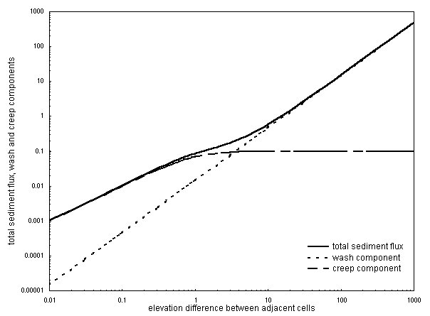
Figure 1. Relationship between elevation difference and sediment flux from originating cell to lowest neighboring cell calculated with Eq. [1] (a = 0.015, b = 1.5 and c = 0.1).
At small values of the elevation difference, small mass movements become the dominant sediment transfer process between cells (Fig. 1). During model runs the maximum sediment flux from an originating cell to its lowest neighbor is kept to less than half the elevation difference between the two cells so that the lowest neighbor cannot become higher than the originating cell in one time step. The maximum sediment flux is determined by the values of a, b and c in Eq. [1]. It is worth noting that the present form of Eq. [1] does not incorporate a threshold elevation difference or slope below which sediment transport ceases. The reason a threshold slope was not used is that the choice of its value has a significant impact on the morphology and structure of the modeled landscape. To avoid dealing with an additional parameter, and to enable the evolution of the modeled landscape towards a peneplain in a fixed baselevel scenario, there is no threshold slope in the model.
At the edge of the grid, sediment yield is calculated in a form of Eq. [1] modified to
F = a SBb + c sin(atn(SB)) [2]
where SB is the elevation difference between the cell on the edge and baselevel. Through time, baselevel is lowered as sediment export occurs, following rule 5.
The objective of the model is not to model the evolution of a specific landscape in order to predict or postdict its sediment transport record. Instead, the objective of the model is to evaluate how local rules of sediment transport result in a global pattern of sediment dynamics. As a result, the spatial and temporal scales of the model need not be strictly defined, other than that in general terms the model concerns large temporal and spatial scales. An important spatial scale consideration is that each cell represents an area with a size of the order of 101 to 102 square kilometers. Thus, the processes in each cell are a combination of channel and slope processes, and no distinction is made between channel and slope cells. In terms of temporal scale, the model is aimed at evaluating landscape evolution and sediment dynamics over periods of 103 to 105 years.
Figure 2 shows an example of an initial landscape (Fig. 2a) and the eroded landscape after 400,000 rainstorms drawn from a rainstorm population in which the probability of a rainstorm is inversely proportional to its area (Fig. 2b).
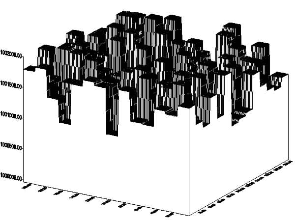
Fig. 2a Initial topography, 210 x 210 cells.
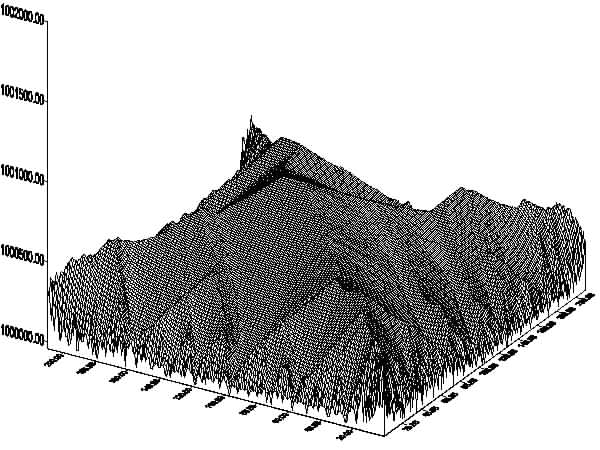
Fig. 2b Topography after 400,000 random rainstorms drawn from a population in which the probability of a rainstorm is inversely proportional to its area. Parameter values as in Fig. 1.
Note that all traces of the initial landscape in Fig. 2a are erased so that the initial conditions are effectively immaterial. A notable feature of Fig. 2b is a narrow, elevated, irregular zone found along the edge. This narrow zone is caused by the small drainage area for the cells along the edge. As a result, these cells receive little water from areas upstream so that relatively little erosion and deposition occurs.
Because of the objective of the model, modeling results cannot be compared with measured values. Instead, model results can be analyzed to evaluate its general features. One of these features is the frequency distribution of total sediment yield (Fig. 3).
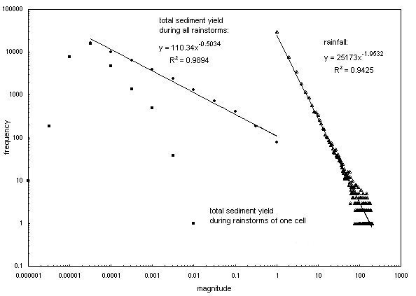
Fig. 3 Frequency distributions of rainstorm area, total sediment yield of all rainstorms and total sediment yield for rainstorms with an area on one cell for 50,000 rainstorms (rainstorm 350,001 to 400,000). Parameter values as in Figure 1.
Sediment yield represents the response of the modeled landscape to an input of rainfall. In the modeling runs discussed here, the rainfall added to a cell was always one unit, which implies that all rainstorms, regardless of storm area, had the same intensity. Figure 3 also displays the frequency distribution of rainstorm area. Because in this model run the probability of a rainstorm is inversely proportional to its area and, the frequency distribution follows a power law with a theoretical value of the exponent of -2. In Figure 3, the frequency distribution has an exponent of -1.95. Analysis of a longer time series would bring the measured value of the exponent closer to the theoretical value. During the model runs, a record was kept of the total sediment load exported from the grid during each rainstorm. Sediment loads were divided into 13 classes with equal widths on a logarithmic scale. As Figure 3 indicates, the frequency distribution of the total sediment yield shows few small loads, many medium loads, and a decrease in frequency of occurrence as the sediment load increases. For the medium to large loads, the relationship between load magnitude and frequency of occurrence is given by a power law with an exponent of -0.50. Model runs were carried out with rainstorm frequency distributions with exponents between -2 and -3. The decrease in the exponent from -2 to -3 indicates that rainstorms with large areas become increasingly rare. As the exponent of the rainstorm frequency distribution decreases to -3, the exponent of the straight section of the total sediment yield frequency distribution decreases to -1.07 indicating that, as expected, large loads also become increasingly rare relative to small total sediment loads.
A graph of rainstorm area and total sediment yield indicates that overall there is a direct relationship between the two variables (Figure 4).
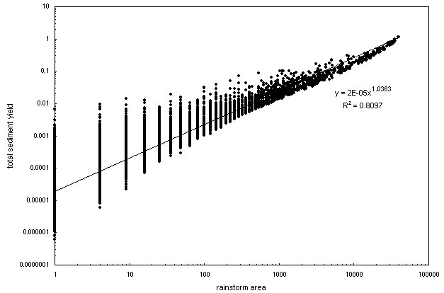
Fig. 4 Relationship between rainstorm area and total sediment yield for 32,000 rainstorms (rainstorm 350,001 to 382,000). Parameter values as in Fig. 1.
The relationship, however, is characterized by a substantial amount of scatter. For the smallest rainstorm area of one cell, for example, the total sediment yield varies over four orders of magnitude. As rainstorm area increases, the range of total sediment yield decreases. This decrease in range is likely due to the smaller number of rainstorms with large areas. The contribution of rainstorms of one cell to the frequency distribution of total sediment yield shows that most small sediment loads are associated with these rainstorms (Fig. 3). As the total sediment yield increases, the contribution of the one-cell rainstorms becomes smaller, and larger sediment loads are exclusively associated with rainstorms with areas greater than one cell.
The temporal pattern of total sediment yield for one-cell rainstorms indicates an absence of temporal trends so that changes in total sediment yield for these storms cannot be attributed to evolution of the modeled landscape; thus, there is no simple one-to-one relationship between rainstorm area and total sediment yield, and instead it appears that landscape response to a rainstorm as indicated by total sediment yield reflects changes caused by erosion and deposition within the landscape during previous rainstorms. To investigate the effect of variations in rainstorm area, model runs were carried out with a constant rainstorm area of one cell. During these runs, total sediment yield did vary over several orders of magnitude. Most values of total sediment yield, however, were clustered around the average and very few large values occurred. The wide range of sediment loads shown in Figs. 3 and 4 can only be reproduced by applying rainstorms of different areas.
The simple rules of sediment transport between adjacent cells in the model give rise to a record of total sediment yield with features, such as its frequency distribution and its range of magnitude, which cannot be predicted from the simple, local rules. The sediment dynamics of the modeled landscape are an emergent property of the entire system resulting from the local interaction of the individual cells. It is tempting to draw an analogy between the sediment dynamics of the modeled landscape and the sediment dynamics of real landscapes. In the latter case, rainstorms of differing area and, in the real case, of differing intensity, occur in the landscape, resulting in erosion and deposition and, ultimately, sediment export from the drainage basin and from the continent into the ocean. In real landscapes, evolution does not follow a master plan but even so, erosion and deposition of the individual particles result in the formation of landscapes with a well-defined and clearly visible morphological structure, and with sediment dynamics reflecting its morphology and history. At present, the link between the sediment dynamics of modeled and real landscapes is not readily made, partly because records of sediment yield are typically available for only relatively short periods. Nevertheless, from this study the following conclusions can be drawn and avenues for further research can be pointed out:
1. The sediment dynamics of a drainage basin are an emergent property of the system itself. Even though the sediment dynamics of a drainage basin result from the small-scale, local processes within the basin, knowledge of these local processes can at best only partly explain the behavior of the system itself. Any understanding of how a drainage basin functions as a system should be developed at the drainage basin level. This point is illustrated by a number of field studies that have indicated that the sediment yield of a drainage basin bears little relation to the amounts of erosion within the basin (e.g. Trimble, 1981, 1983). Future research on the sediment dynamics of drainage basins should continue to take a holistic view of the drainage basin rather than concentrate on the microscale details of sediment transport.
2. The relationship between sediment load magnitude and frequency of occurrence is one of the properties of the sediment yield record that can be analyzed to provide information on how a drainage basin functions as an integrated system. Since total sediment yield is the response of the landscape to an input of rainfall, the frequency distribution of rainstorm size affects the frequency distribution of total sediment yield; nevertheless, there is no one-to-one relationship between the magnitude of an individual event, i.e., the rainstorm, and the response of the drainage basin to this event, i.e., total sediment yield. Instead, the response of the drainage basin depends, to a certain extent, on its recent history in terms of rainstorm area, rainstorm location, and total sediment yield. Future research should be directed towards evaluating the long-term statistical properties of sediment loads, discharges, and rainfall.
3. In the model, chance plays a role as the area and location of rainstorms are selected at random. Over the long run, however, the impact of each individual rainstorm becomes negligible as it is erased by subsequent rainstorms, and instead, the frequency distribution of, in these model runs, rainstorm area becomes the crucial factor. Duplicate model runs with different starting points for the random number generator results in only minor differences in topography and sediment dynamics as indicated by the frequency distribution of total sediment yield. At any given time, however, plots of rainfall and total sediment yield against time are completely different between the duplicate model runs, emphasizing that the model described here is not designed for predicting sediment loads, but instead for evaluating how the simple, local rules of sediment become integrated at the drainage basin level over the long term.
Armstrong, A., 1976. A three-dimensional simulation of slope forms. Z. Geomorph. N.F., Suppl. Bd. 25, pp. 20-28.
Armstrong, A.C., 1987. Slopes, boundary conditions, and the development of convexo-concave forms - some numerical experiments. Earth Surface Processes and Landforms, 12, pp. 17-30.
Bak, P., 1996. How Nature Works. Springer-Verlag, New York, NY.
Bak, P., C. Tang and K. Wiesenfeld, 1988. Self-organized criticality. Physical Review A, 38, pp. 364-374.
Chase, C.G., 1992. Fluvial landsculpting and the fractal dimension of topography. Geomorphology, 5, pp. 39-57.
Favis-Mortlock, D., T. Guerra and J. Boardman, 1998. A self-organizing dynamic systems approach to hillslope rill initiation and growth: model development and validation. International Association of Hydrological Sciences Publication 249, pp. 53-61.
Forrest, S.B. and P.K. Haff, 1992. Mechanics of wind ripple stratigraphy. Science, 255, pp. 1,240-1,243.
Kirkby, M.J., 1976. Deterministic continuous slope models. Z. Geomorph. N.F., Suppl. Bd. 25, pp. 1-19.
Kirkby, M.J., 1984. Modelling cliff development in South Wales: Savigear re-viewed. Z. Geomorph. N.F., 28, pp. 405-426.
Leopold, L.B. and W.B. Langbein, 1962. The concept of entropy in landscape evolution. U.S. Geological Survey Professional Paper 500-A, p. 20.
Murray, A.B. and C. Paola, 1994. A cellular model of braided rivers. Nature, 371, pp. 54-57.
Murray, A.B. and C. Paola, 1996. A new quantitative test of geomorphic models, applied to a model of braided streams. Water Resour. Res., 32, pp. 2,579-2,587.
Murray, A.B. and C. Paola, 1997. Properties of a cellular braided-stream model. Earth Surf. Process. Landf., 22, pp. 1,001-1,025.
Rodriguez-Iturbe, I. and A. Rinaldo, 1997. Fractal River Basins: Chance and Self-Organization. Cambridge University Press, Cambridge.
Trimble, S.W., 1981. Changes in sediment storage in the Coon Creek Basin, Driftless Area, WI, 1853 to 1975. Science, 214: pp. 181-183.
Trimble, S.W., 1983. A sediment budget for Coon Creek Basin in the Driftless Area, WI, 1853-1977. Am. J. Sci., 283: pp. 454-474.
Werner, B.T. and T.M. Fink, 1993. Beach cusps as self-organized patterns. Science, 260, pp. 968-971.
Werner, B.T. and B. Hallet, 1993. Numerical simulation of self-organized stone stripes. Nature, 361, pp. 142-145.