Return to GeoComputation 99 Index
Paul Crowther, Jacky Hartnett, and Ray Williams
University of Tasmania, School of Computing, P.O. Box 1214, Launceston, Tasmania 7250 Australia
E-mail: P.Crowther@utas.edu.au
Steve Pendelbury
Bureau of Meteorology
One of the strengths of a remotely sensed data set is that it represents a complete spatial population; however in order to make sense of this population the most successful classifiers first require areas of the image be selected as training data. This paper describes a method that solves the problem of selecting suitable training sites when it is not practical to select these using ground truth. The method was developed to provide a training data set for a statistical decision tree classifier to analyse NOAA AVHRR multispectral satellite images of Antarctica. This was in response to a user request for a tool to develop a data set for a statistical decision tree package, "S-Plus" (Chambers and Hastie, 1992). It was then found that the same tool could be used to create training data for use with other systems.
This paper will describe the operation of the spatial sampling tool and the results of using the sample to develop a decision tree by submitting this sample to the S-Plus decision tree package. The results of applying this decision tree to classify Antarctic sea-ice will be presented.
Statistical classifiers are dependent for their accuracy on the quality of the training data as much as on the algorithm used for classification. For useful results to be obtained, the training data set must be representative of the whole area to be classified. The populations of pixels used for training must be statistically significant. This means that there is a need to know the minimum number of observations required to characterise a particular site to an acceptable level of error.
Ground-truthed training data in Antarctica is difficult to obtain. In other domains, for example vegetation classification, training data are developed using ground truth combined with aerial and satellite interpretation to identify representative vegetation types. Vegetation also is relatively stable over time. In Antarctica there can be rapid changes in features such as sea ice that cannot be easily verified on the ground. Training data therefore must be developed directly from satellite images.
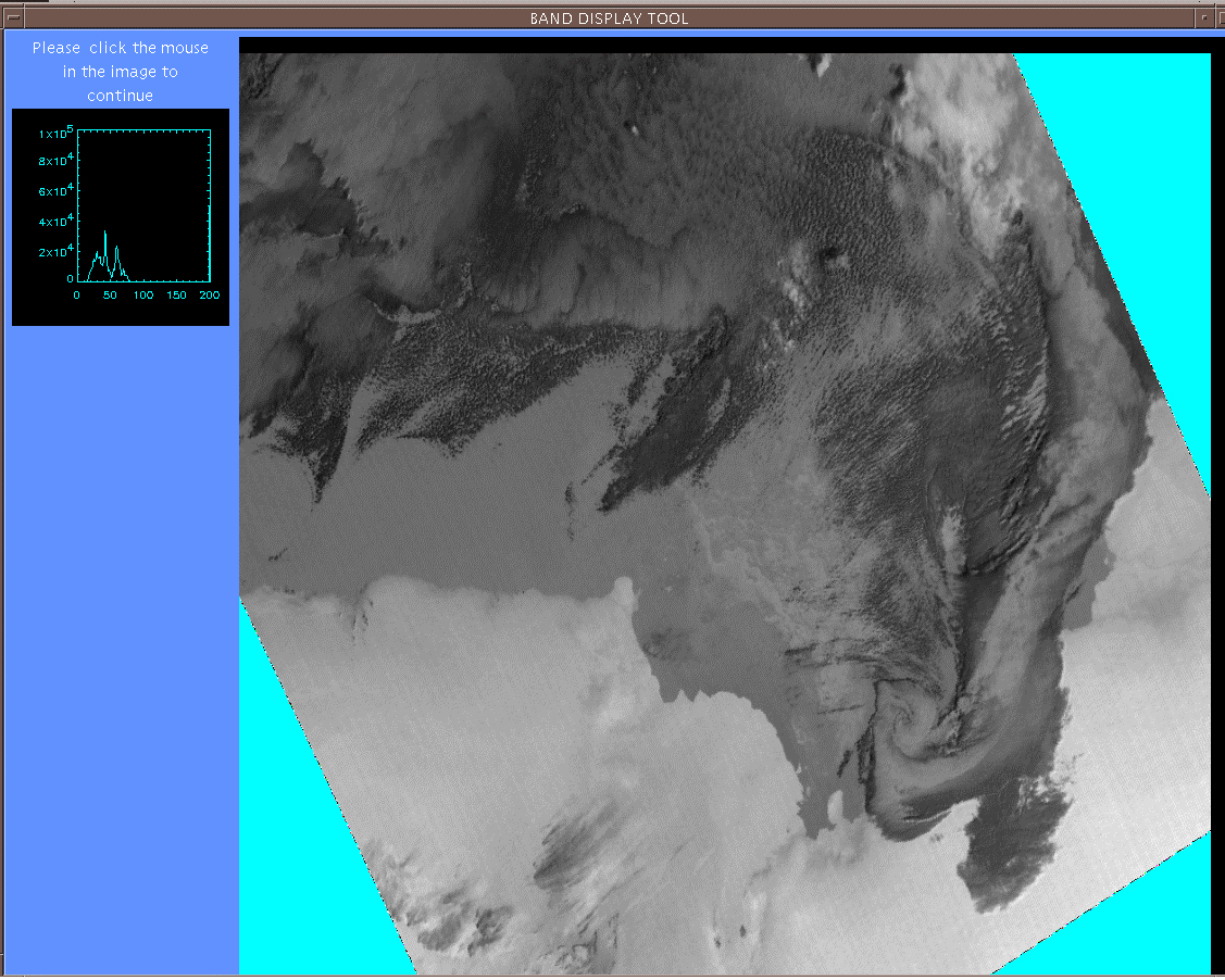
In this paper there will be a discussion on acquiring training data for the statistical decision tree package S-Plus. This has been used to develop rules for classification of Antarctic NOAA AVHRR images (Figure 1). The purpose of this classification is to identify areas of low concentration ice that can be navigated by resupply vessels as well as to determine the extent of pack ice for climate studies.
Figure 1: Thermal band 3 of the test image, derived from a NOAA AVHRR image of Mawson/Davis taken on 4 March 1998 viewed using the KAGES (Crowther and Hartnett, 1997) band display tool.
The accuracy of the classification of satellite images that result from the use of supervised statistical techniques depends on the quality of the training data used rather than the actual classification algorithm (Buttner et al., 1989). Although remote-sensing software contains classification algorithms, their success depends basically on the quality of the training data sets.
Supervised classification of multispectral data requires the selection of a number of training pixels in an image. These pixels belong to a class of land cover that is known, and to which a name or label can be attached. Generally a number of training pixels of the same class will be chosen to describe the spectral range of the class. The values of these pixels will vary, but usually range within a discrete cluster of values (Molenaar, 1988).
It is important that training pixels be representative of the whole class, but at the same time include a range of variability for the class (Schowengerdt, 1997); that is, the training data must be representative and complete. Lillesand and Kiefer (1994) state that the minimum number of pixels required for a training set is n + 1 where n is the number of spectral bands and at least one pixel is from each band; however, they continue to add that in practice, a minimum of 10n to 100n should be used for improved statistical representation.
S-Plus was chosen as a package to derive a decision tree for classification of Antarctic scenes. This classifier required a complete representative spatial sample.
Training data are usually selected on the basis of ground truth. Training samples are selected from those sites that can be extensively investigated (Curran and Williamson, 1986). This would involve a field survey of the actual ground cover near the time of the image acquisition. There are cases where this is not practical, in Antarctica, for example. Here, even airborne surveys are difficult to obtain, especially during the Antarctic winter. As a result, the only effective way to develop training data is to rely on expert interpretation of satellite images.
The image interpretation expert generally classifies images by manually delimiting objects and assigning them a label. To do this they may change between image bands, or use some combination of bands. For example, the combination of bands B2 ó B1 is used to determine if there is ice under cloud based. This has problems, in that an expert interpreter can rarely work with more than two image bands (or composite bands) simultaneously.
The expert user can perform data sampling for the S-Plus tool manually. This involves picking training points on the image that are considered representative of object classes, then manually noting the pixel values and locations from those points from several image bands. The experts stop collecting these data when they have collected a representative sample.
Knowledge Acquisition for Geographic Expert Systems (KAGES) is a toolkit containing a number of tools for knowledge acquisition from experts who interpret satellite images (Crowther and Hartnett, 1997). The Point Data Tool allows an image interpreter to create training data at various locations across an image without the need to manually record data values. This is done in either automated sampling mode or manual mode. In automated mode, the system asks the user to select the sampling density using slider bars to define the granularity of the sampling grid. The system then samples the image set using the sampling grid and requests the user to name the sample points. Using this method an appropriate sample grid can be determined and the user directed to construct a training sample.
The automated mode may miss sampling some classes that are present on an image. This is because there are either very few of them or the sampling grid may have been set too coarse; therefore there is a facility to allow a user to manually sample objects that have been "missed" by the grid.
In manual mode the system operates in a similar manner to the automated mode, but unconstrained by the sampling grid. It allows the user to select the points on the image to be named. A typical user would start with the regular grid then complete the data set by sampling "missed" features in manual mode.
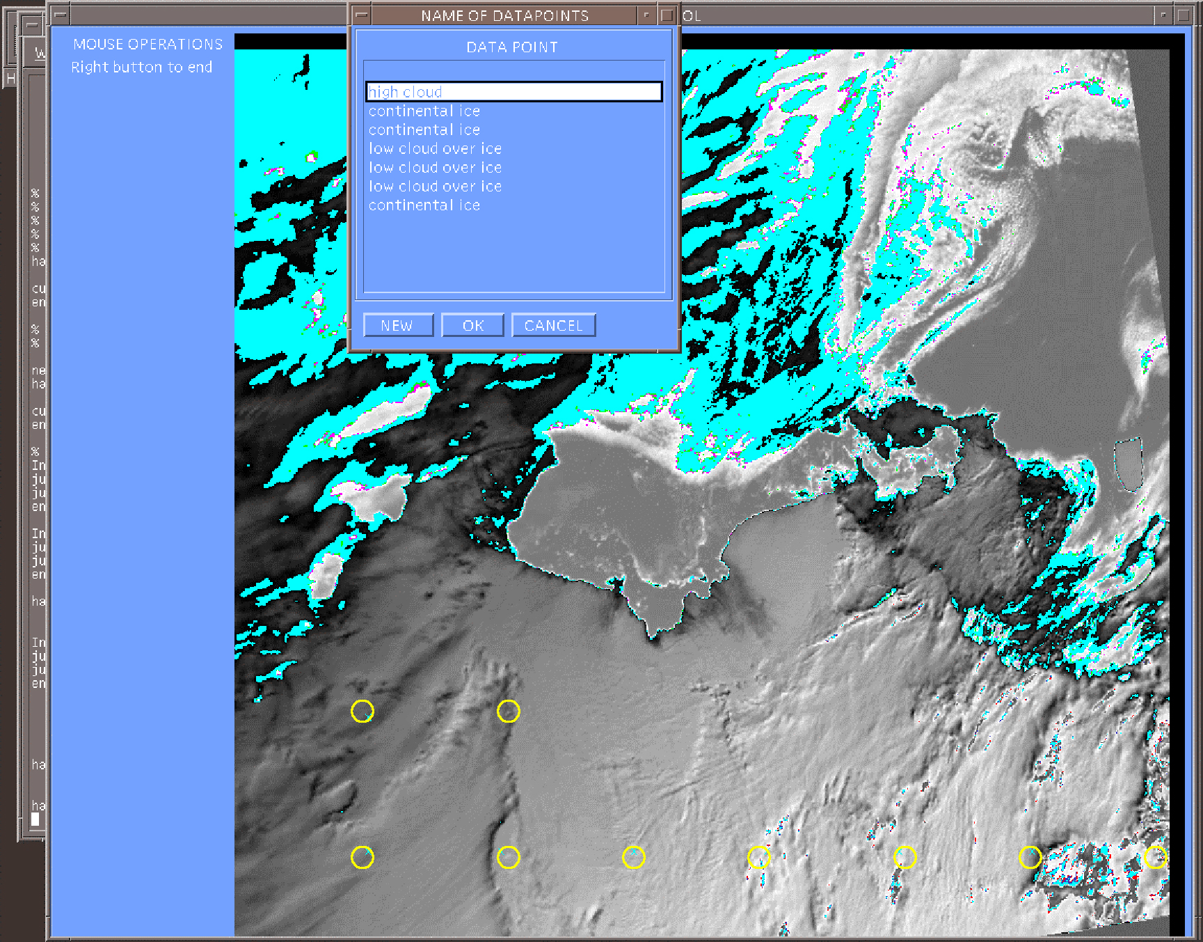
Figure 2: Point data tool showing sampling points designated by O on the training image and the naming window (NOAA VHRR image of Casey taken on 26th February 1998).
As each point is selected either by the system or the user, the user is requested to name the class of point it represents. To do this, a user can select a previously entered label or enter a new label for the sample point. The system then records the pixel values on all bands of the image at that point, the location of the pixel and the label.
At any time during the development of the training data the user has the option to:
The saved data are held in a form similar to Table 1. This data file can be combined with other files containing further training data in order to make a complete training set.
BAND Location
| 1 | 2 | 3 | 4 | 5 | class | X | Y |
| 141 | 127 | 4 | 85 | 85 | high cloud | 127 | 128 |
| 153 | 137 | 48 | 79 | 80 | continental ice | 254 | 128 |
| 166 | 146 | 27 | 75 | 75 | continental ice | 381 | 128 |
| 159 | 137 | 13 | 77 | 77 | low cloud over ice | 508 | 128 |
| 178 | 155 | 17 | 80 | 80 | low cloud over ice | 635 | 128 |
| 143 | 122 | 12 | 76 | 79 | low cloud over ice | 762 | 128 |
| 139 | 115 | 41 | 67 | 68 | continental ice | 889 | 128 |
Table 1: sample of a typical training set created by the KAGES sampling tool.
The original method of developing training required the user to make a pen and paper note of values at various pixel values and their locations on an image. This was then entered via keyboard into a computer file that was used as input for S-Plus. This took the user approximately 8 hours. By using the sampling tool this process was reduced to 2 hours and reduced the possibility of errors since there was no manual transcription.
The sample data were used to train the S-Plus decision tree and the resulting rules were applied to other images. The resulting classification was then compared with that derived from rules obtained using traditional knowledge engineering techniques.
This alternative approach to developing a classifier used an expert system with a rule-based per-pixel classifier where an expert image interpreter provided the rules. These rules were acquired during interviews and demonstrations. Information normally acquired as training data is acquired as spectral thresholds. These are then applied to an image. Such a system, known as Icemapper, was developed for ice classification (Williams et al, 1997). One problem with this method of knowledge acquisition is that it is time consuming and subject to error caused by the interviewer misunderstanding the image classifier's methods. This is a problem common to many expert interpretation systems and has been termed the knowledge acquisition bottleneck (Cullen and Bryman, 1988).
|
High |
109 |
|
Low |
52 |
|
Continental |
80 |
|
Pack |
52 |
|
Water |
38 |
|
Rock |
7 |
|
|
|
|
Total |
338 |
Table 2: Training data
Three hundred thirty eight usable sample points were acquired from a training image and are shown in Table 2. It should be noted that this image contained an area free of ice (rock) that did not exist in the test image.
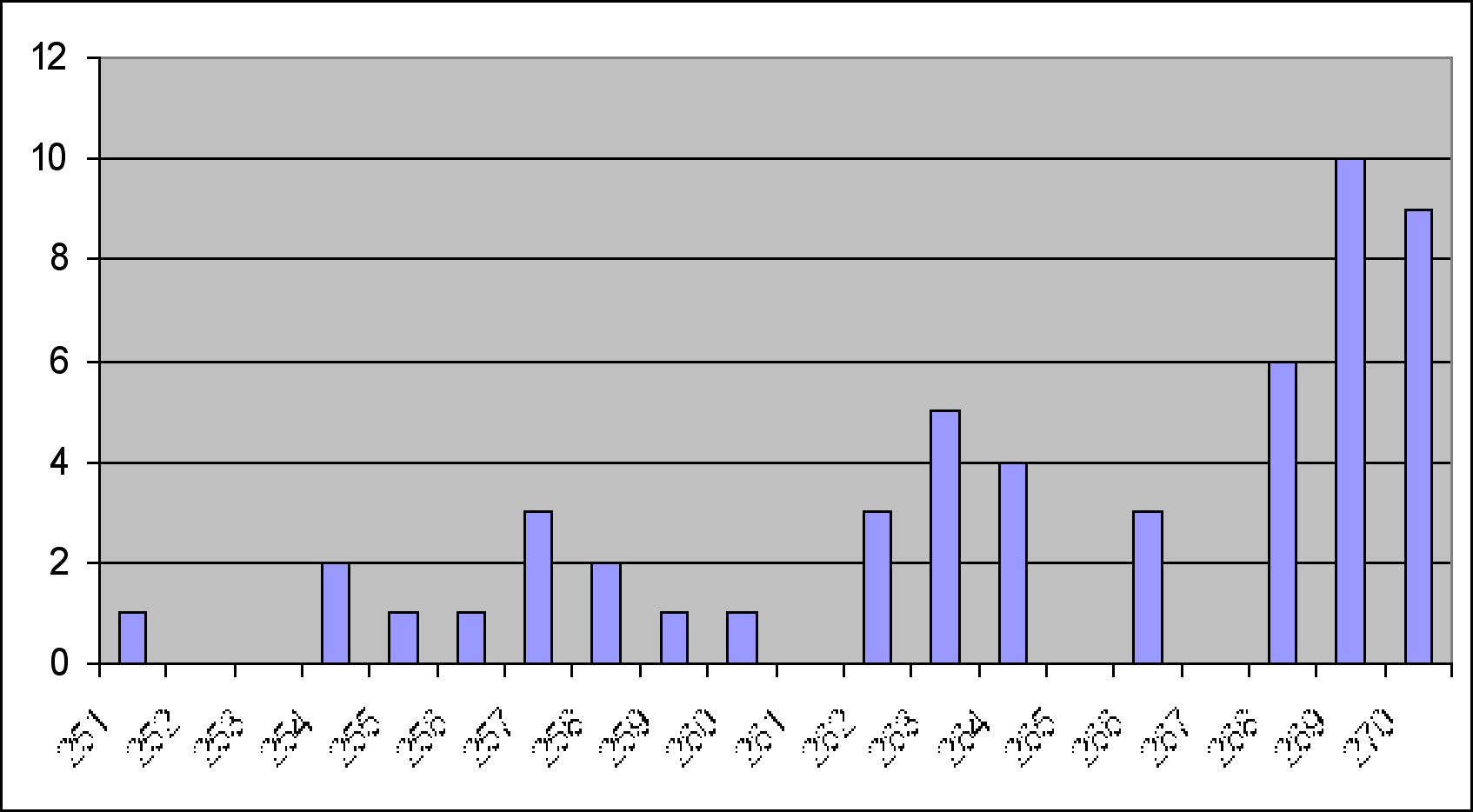
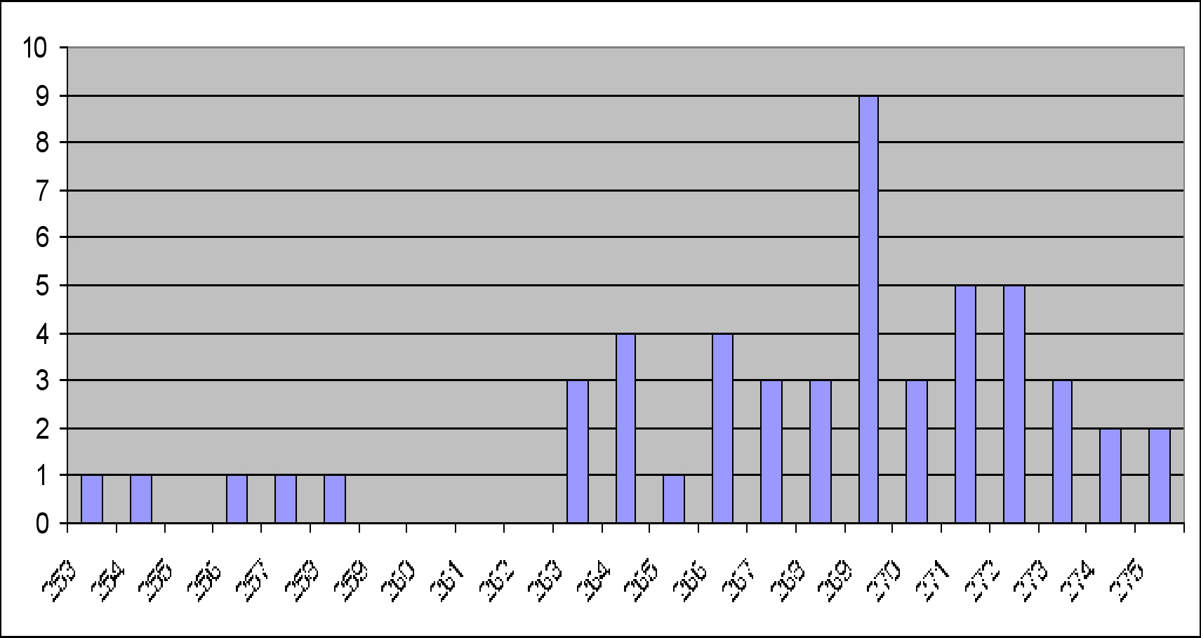
Figures 3 and 4 show histograms of the range of pixel values sampled in the training image sampled as class pack ice for bands T3 and T4. It is interesting to note the existence of outlier pixel values at the lower end of the scale. The pixels involved correspond on both image bands. They may be due to the expert image interpreter assigning a label to a pixel that is not representative because of noise caused by some other class. In other words, a mixed pixel has been selected.
Figure 3: Histogram of the class ëpack-iceí from band T4.
Figure 4: Histogram of class ëpack-iceí from band T3.
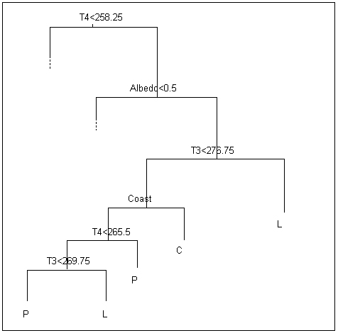
Pack-ice (labelled P) identification is achieved using the segment of the decision tree generated by S-Plus shown in Figure 5. From this figure it can be seen that the package has ignored the outlying pixel values. In the case where T4 is greater than 258.25, there is a segment of the tree that is not shown that follows the path of T3<270.25, then T4<250, which also results in a classification of pack-ice.
Figure 5: Segment of the decision tree produced using the training data. P=pack-ice, C=continental ice, L=low cloud.
|
|
SAMPLE |
S |
ICEMAPPER |
|
HIGH CLOUD |
105 |
47% |
0% |
|
LOW CLOUD |
31 |
90% |
90% |
|
CONTINENTAL ICE |
167 |
98% |
94% |
|
PACK ICE |
8 |
100% |
88% |
|
THIN CLOUD OVER ICE |
72 |
71% |
39% |
|
WATER |
84 |
95% |
99% |
|
THIN HIGH CLOUD OVER ICE |
167 |
65% |
5% |
|
|
|
|
|
|
OVERALL |
634 |
77% |
49% |
Table 3: Comparison of Icemapper and S-Plus performance on the test image
In the final classification, further processing was carried out on areas labelled cloud to determine the presence of ice under the cloud. This was not part of the decision tree but the results of this have been added to Table 3.
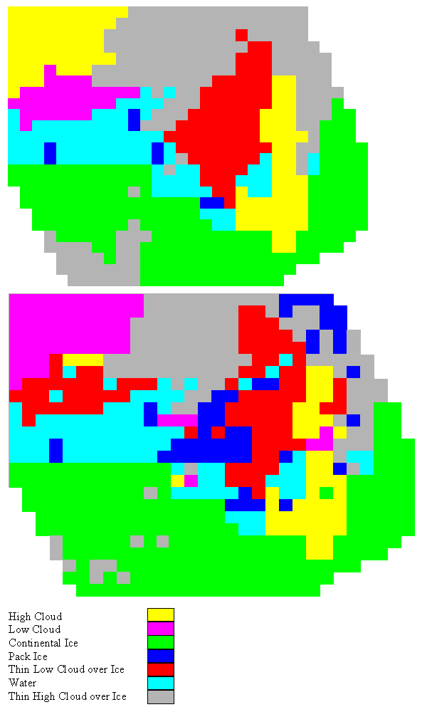
Figure 6: Comparison of expert classification (upper) and S-Plus rule classification (lower) at sample points across the image
To test the accuracy of the rules developed from S-Plus, the results of classifying the image shown in Figure 1 were compared with the results of using the Icemapper rules and the results of a manual classification by an image interpretation expert. A regular sampling grid of 634 points across the image was used to compare the expert's classification with the two systems. The results are presented in Table 3 and Figure 6.
Generally, the S-Plus rules performed well, thus indicating a useful set of training data were developed with the KAGES sampling tool. Most misclassifications were for ice under cloud (which was classified using an algorithm not derived from the training pixels). The main misclassification was an area of cloud in the top right quadrant of the image. This was classified as pack ice when it should have been low cloud. An area of high cloud in the top left of the image was classified as low cloud.
Manual development of training data sets is a time consuming exercise. Where ground truth cannot be easily obtained it also is reliant on expert interpretation of images. This training set development requires the interpreter to note information about pixel values, the pixel location, and a label for the pixel. This information needs to be transcribed to a computer file. In addition to being time consuming, this process also is error prone.
The KAGES sampling tool provides an interpreter with a regular grid sampling tool that can have its granularity adjusted to suit the image being sampled. Supplementary points can be obtained by the user to manually position a pointing device on the image. The user is required to enter a label for the point, information about that pixel, and its location is automatically recorded. This saves time and avoids transcription errors. Data sets derived in this way can be used to train statistical classifiers.
The work reported in this paper has been supported by an Antarctic Science Advisory Committee Research Grant (Project number 2035).
Buttner, G., T. Hajos and M. Korandi, 1989. Improvements to the Effectiveness of Supervised Training Procedures, International Journal of Remote Sensing, Vol. 10, No. 6, pp. 1,005 - 1,013.
Chambers, J. M. and T.J. Hastie, 1992. Statistical Models in S, Wadsworth and Brooks, Ch. 9.
Crowther, P. and J. Hartnett, 1997. Eliciting Knowledge with Visualization - Instant Gratification for the Expert Image Classifier Who Wants to Show Rather than Tell. Proceedings of GeoComputation 1997, Otago, New Zealand.
Cullen, J. and A. Bryman, 1988. The Knowledge Acquisition Bottleneck: Time for Reassessment, Expert Systems, Vol. 5, No. 3, pp. 216 - 225.
Curran, P. J. and H.D. Williamson, 1986. Sample Size for Ground and Remotely Sensed Data, Remote Sensing of the Environment, Vol. 20, pp. 31 - 41.
Lillesand, M. T. and R.W. Kiefer, 1994, Remote Sensing and Image Interpretation (3rd edition), John Wiley and Sons.
Schowengerdt, R. A., 1997, Remote Sensing, Models and Methods for Image Processing (2nd edition), Academic Press.
Molenaar, M., 1988, Key Issues in Image Understanding in Remote Sensing, Phil. Trans. R. Soc. London, A 324, pp. 381 - 395.
Williams, R. N., P. Crowther, and S. Pendlebury, 1997, Design and Development of an Operational Ice Mapping System for Meteorological Applications in the Antarctic, Proceedings of the International Geoscience and Remote Sensing Symposium, Singapore.