Return to GeoComputation 99 Index
Greg Tucker, Nicole Gasparini, Rafael Bras, and Scott Rybarczyk
Massachusetts Institute of Technology, Department of Civil and
Environmental Engineering, Building 48, Room 429, Cambridge, MA 02139 U.S.A.
E-Mail: gtucker@mit.edu
Stephen Lancaster
Oregon State University, Department of Geosciences,
Forest Sciences Laboratory, 3200 SW Jefferson Way, Corvallis, OR 97331 U.S.A.
A number of different strategies have been used for terrain discretization, including regular grids, triangulated irregular networks (TINs), sub-watersheds, contour elements (e.g., Moore et al., 1988), and hillslope partitions (e.g., Band, 1989). Among these, only regular grids and TINs are well suited for simulating the dynamics of surface change. The simplicity of regular grids and the increasing availability of grid-based digital elevation models (DEMs) have made fixed grids the framework of choice in most hydrologic models and nearly all geomorphic models. However, grid-based discretization schemes suffer from a number of distinct disadvantages: (1) landform elements must be represented at a constant spatial resolution, which in practice means the highest resolution required by any feature or process of interest; (2) drainage directions are restricted to 45-degree increments (though for watershed-scale applications, this limitation may be reduced by using multiple-flow algorithms, e.g., Freeman, 1991; Quinn et al., 1991; Costa-Cabral and Burgess, 1994; Tarboton, 1997); (3) under certain circumstances, use of a regular grid introduces anisotropy that can lead to bias in simulated drainage network patterns (Braun and Sambridge, 1997); and (4) use of a fixed grid makes it difficult or impossible to model geologic processes that have a significant horizontal component, such as stream meandering or fault displacement.
The last of these constraints is especially significant in the context of geological models. Although we conventially speak of "uplift," most crustal deformation processes involve a significant amount of horizontal translation. Previous coupled models have either incorporated only the vertical component of deformation (e.g., Tucker and Slingerland, 1996; Kooi and Beaumont, 1996) or have represented lateral translation by simply offsetting two fixed grids (e.g., Anderson, 1994). Coupled models of deformation, erosion, and sedimentation promise to yield important insights into such issues as the relationship between tectonic behavior and the stratigraphic record, but such models ultimately require the ability to model deformation in three dimensions. Similarly, erosional processes often have a significant horizontal component that is neglected in current models. One of the most important horizontal erosion processes is lateral stream erosion, which by widening a valley can signicantly alter the depositional geometry within a floodplain over geologic time.
These and other disadvantages have motivated the development of terrain models based on TINs, which allow for variable spatial resolution, lend themselves naturally to interpolation procedures (e.g., Sambridge et al., 1995), and make dynamic rediscretization a real possibility (e.g., Braun and Sambridge, 1997; Lancaster, 1998; Lancaster et al., in prep). Despite these advantages, however, use of TIN-based dynamic models has not been widespread, in part because of the increased complexity of data structures and algorithm development in a TIN framework. In this paper, we present an efficient set of data structures and algorithms for TIN-based modeling using the Delaunay triangulation criterion. These data structures and algorithms take advantage of the unique capabilities of object-oriented programming languages such as C++ to provide a general framework for (1) storing and rapidly accessing information about mesh connectivity, (2) constructing and updating mesh geometry, (3) computing mass fluxes and maintaining continuity of mass within mesh elements using a finite-difference approach, and (4) establishing drainage pathways across the terrain surface. We present example applications and briefly discuss the use of adaptive meshing to simulate lateral stream channel migration.
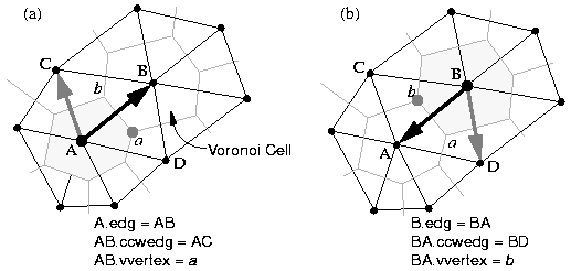
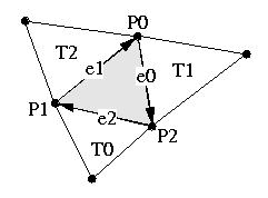
A number of methods for triangulating a set of irregularly-spaced points have been proposed. Here, we focus on the commonly used Delaunay triangulation, which offers a number of distinct advantages over other tesselation schemes (Watson and Philip, 1984). Delaunay triangulations and their corresponding Voronoi diagrams are well established in the field of computational geometry (e.g., Guibas and Stolfi, 1985; Sloan, 1987; Knuth, 1992; Sugihara and Iri, 1994; Sambridge et al., 1995; Du, 1996). The Delaunay triangulation of a set of points Ni is a unique triangulation having the property that a circle passing through the three points of any triangle will encompass no other points. A Delaunay triangulation therefore minimizes the maximum interior angles, providing the most "equable" triangulation of a given set of points. From any Delaunay triangulation it is also possible to construct a unique corresponding Voronoi (or Thiessen) diagram, which is the set of polygons formed by connecting the perpendicular bisectors of the triangles (Figure 1). Although Voronoi polygons have been ignored in most TIN-based models, they have the advantage of providing a natural framework for finite-difference modeling.
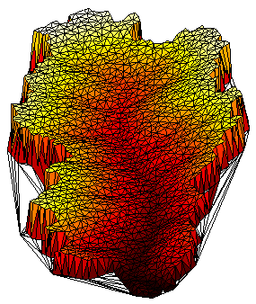
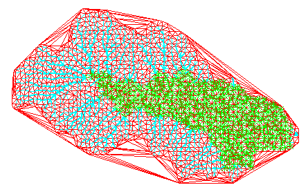
A simulated terrain using a triangular discretization is shown in Figure 2. As with Braun and Sambridge (1997), the model in this example uses a finite-difference rather than a finite-element approach, in which state variables such as elevation and water flow are computed at the nodes rather than within the triangles. The data structure developed below is thus designed with finite-difference modeling in mind, though in principle it could be easily applied to finite-element applications. The terrain is represented by a set of nodes N that are connected to form a mesh of triangles using the Delaunay triangulation of N. Each node Ni is associated with a Voronoi polygon of area (Figure 1). The Voronoi polygon for a node Ni is the region within which any arbitrary point Q would be closer to Ni than to any other node on the mesh. The boundaries between Voronoi polygons are lines of equal distance between adjacent nodes, and coincide with the perpendicular bisectors of the triangle edges. The vertices of the Voronoi polygons (here termed Voronoi vertices) coincide with the circumcenters of the triangles; in general, each triangle is associated with one and only one Voronoi vertex.
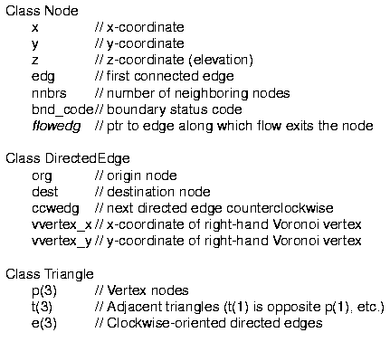
Unlike regular matrices, in which each node is connected to either four or eight adjacent neighbors, the number of neighbors connected to a given node in a Delaunay triangulation may in theory be arbitrarily large. Ideally, a data structure should represent this variable connectivity in a way that (1) provides rapid access to adjacent mesh elements without demanding excessive storage space, and (2) is flexible enough to handle dynamic changes in the mesh itself. For dynamic modeling applications, an additional requirement is the need to maximize computational speed. These requirements are satisfied through the use of the following data structure. The "Dual Edge" structure is adapted from the Quad Edge data structure of Guibas and Stolfi (1985), and consists of three geometric elements: nodes, triangles, and directed edges. The data structure is summarized in pseudo-code form in Figure 3.
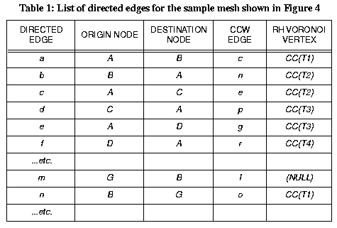
Each directed edge data object also includes the coordinates of the Voronoi vertex associated with the triangle on its right-hand side (clockwise) (Figure 1). Pseudo-code for the DirectedEdge data structure is given in Figure 3, and an example list of edges for a simple mesh is given in Table 1. Complementary directed edges are stored pairwise on the list (Table 1), which makes it possible to quickly retrieve the complement of any given edge. In addition, certain operations such as length and slope calculation only need to be performed for one member of each edge pair, with the result simply assigned to the other. Storing directed edges pairwise makes it possible to do this easily by skipping every other edge on the list. In addition to topologic information, a directed edge object might include geometric properties such length, gradient, and the length of the associated Voronoi polygon edge (or Voronoi edge).
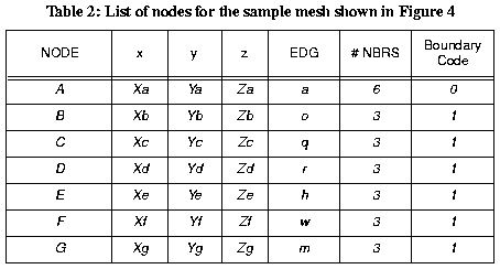
For finite-difference applications, a node object can also include geometric information such as the projected surface area of its Voronoi polygon (Voronoi area) and a flag indicating whether it lies on the boundary or interior of the mesh. An important advantage of an object-oriented programming language in this regard is that basic topologic and geometric data and functions can be encapsulated within a base class, with application-specific data and functions added as part of an inherited class. This technique is exploited in the examples discussed below.
Generally, neighbor node and spoke list retrieval would be handled separately; they are grouped here for simplicity. Note that creating a list (as opposed to simply performing operations on each spoke in turn) is usually not necessary, though it may be convenient for performance reasons. The same basic algorithm can be used to sweep through each neighbor node to perform any operation.
Once the Voronoi vertex coordinates have been stored, the Voronoi polygon for a given node can be retrieved using the following simple algorithm:
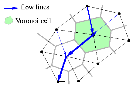
Here, we describe a simple "Voronoi-based" approach to routing that avoids these problems, though at the expense of added simplicity. Following Braun and Sambridge (1997), flow originating at any point within a node's Voronoi polygon is routed downslope along the steepest of the spokes connected to that node (Figure 6). By this method, the contributing area at node i is equal to the sum of the Voronoi areas of all nodes that flow to i (including i itself). An advantage of this approach is that it lends itself to finite-difference modeling, because each node has a unique watershed and drainage direction assigned to it. The primary disadvantages are: (1) drainage basin boundaries are defined by Voronoi polygons rather than by triangles, and (2) flow pathways and gradients are forced to follow triangle edges. The second limitation could be eliminated by adopting a more general flow routing procedure (e.g., Tarboton, 1997), though such an extension is beyond the scope of this paper.
To identify flow directions, the steepest spoke at each node is identified and a pointer to it is stored in node.flowedg (Figure 3). The total contributing area for each node can then be found using the following algorithm:
During the process of identifying flow directions, any node lacking a downhill pathway is flagged as a pit. Once all pits have been identified, the FillLakes algorithm (Appendix A) is invoked for each one. The algorithm begins by creating a list of flooded nodes, which initiatially contains only the starting pit. The lowest node on the perimeter of the flooded area ("lake") is identified, and is tested to see whether it can drain downslope toward a node that is not already on the list. If there is no drainage outlet, this "low node" is added to the list of flooded nodes and the process repeats, continuing until an outlet is found. If a node is encountered that is part of separate lake (i.e., one identified during a previous iteration), it is also added to the list (in other words, initially separate lakes can merge).
Once an outlet has been identified, all of the nodes on the list are flagged as lake nodes, indicating, for example, that they should be handled separately in computing runoff and sediment routing. To maintain the continuity of drainage networks, flow directions for lake nodes can be resolved by iteratively tracing a flow path upstream from the lake outlet, seeking the shortest path to the outlet for each node (Appendix B). Once flow directions have been resolved, the lake list is cleared and the next pit is processed.
An example of a lake computed using the Lake Fill algorithm is shown in Figure 7. The algorithm is robust enough to handle any arbitrary initial condition, and is useful for modeling natural or artificial reservoirs or, in geological applications, for modeling rising baselevel.
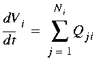
where Vi represents volume or mass stored at node i, Ni is the number of neighbor nodes connected to node i, and Qji is the total flux from node j to node i (negative if the net flux is from i to j). Numerical implementation of equation (1), however, depends on how the flux terms are defined.
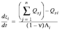
where zi is the elevation at node i, t is time, n is the number of nodes that flow directly to i, Qs is sediment flux, n is sediment porosity, and /\i is the Voronoi area of node i (Braun and Sambridge, 1997; Tucker et al., 1997). The system of ordinary differential equations described by equation (2) can be solved using simple forward differencing, via matrix methods, or by any similar scheme. Solving equation (2) in upstream-to-downstream order ensures that the total incoming sediment flux at any point is always known.
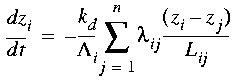
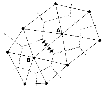
where kd is a diffusivity constant and x' is a vector orientated in the downslope direction. To solve this equation in a TIN framework, the slope width between two adjacent nodes can be approximated by the width of their shared Voronoi cell edge, lij (Figure 8). Combining this with continuity of mass (equation (1)), the rate of elevation change at a node due to diffusive transport is approximated numerically by
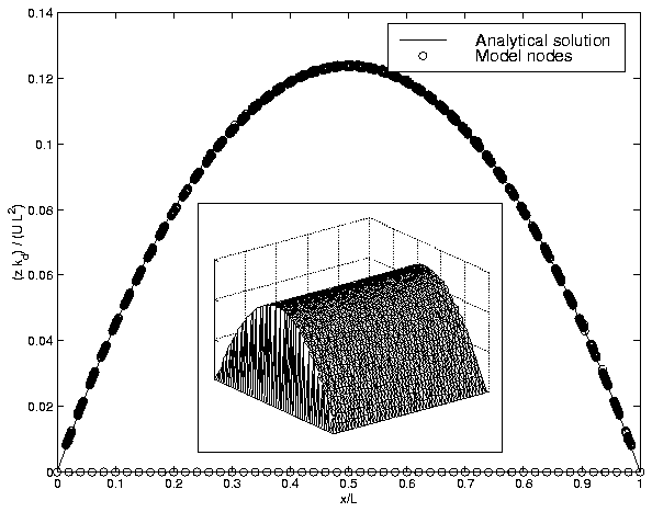
where n is the number of nodes adjacent to node i, Lij is the length of the triangle edge connecting nodes i and j, and lij is the width of the shared Voronoi cell edge between nodes i and j. In the CHILD model (Tucker et al., 1997), this system of equations is solved using a simple forward-difference method with an adaptive time-stepping scheme. Note that because diffusive mass exchange takes place along triangle edges, the equation can be solved efficiently by first computing the mass exchange along each physical edge (or equivalently, across each Voronoi polygon face), then updating the node elevations accordingly. This numerical algorithm performs well when compared with analytical solutions (Figure 9).
Similarly, 2D groundwater flow can be approximated numerically using an expression of the following form:
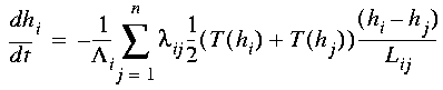
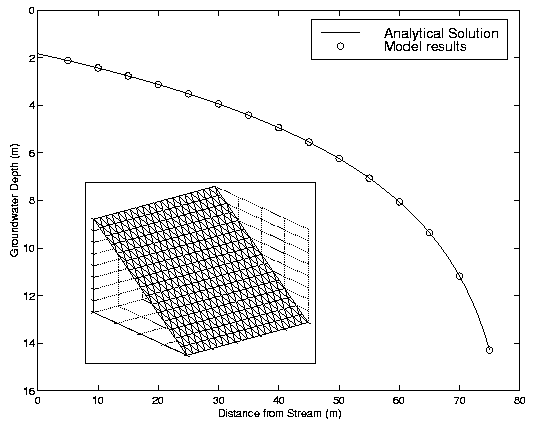
where hi is the groundwater table elevation at node i and T(hi) is transmissivity (in this example, transmissivity is assumed to vary with water table height, with the average transmissivity between nodes i and j used to compute the flux between them). Figure 10 compares the equilibrium water table height as computed from a simplified version of equation (5) with an analytical solution, assuming a simple linear hillslope geometry.
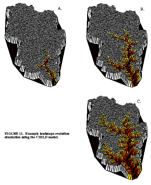
Figure 12 illustrates a hydrologic application of the same concepts. The figure shows simulated depth to the water table in a small catchment in Kansas in response to spatially uniform recharge. Water table depth at each point is computed using eq (5), assuming an expontial decrease in saturated hydraulic conductivity with depth. In both of these examples, the TIN framework is implemented in C++, with each data element (nodes, triangles, and directed edges) encapsulated within a single class. The hydrologic model and the landscape evolution model (Figure 11) use the same code for mesh handling and drainage network delineation, which highlights the advantages of a modular, object-oriented approach in terms of code reusability.
The data structures and algorithms we have outlined are also well suited to applications involving dynamic remeshing in response to changing surface morphology. Figure 13 illustrates output from a model that combines vertical erosion/deposition with lateral erosion associated with river meandering. Such adaptive remeshing strategies make it possible to explore a range of geologic problems that were heretofore inaccessible to modeling, such as horizontal tectonic deformation. The adaptive meshing strategy is discussed further by Lancaster (1998) and Lancaster et al. (in prep).
The data structure also simplifies bookkeeping. Each node points to a single directed edge (or spoke), which then points to its counterclockwise neighbor, thus fully describing the connectivity between nodes and triangle edges. The data structure also contains sufficient information to provide a complete representation of Voronoi geometry.
Based on this framework, we describe a simple flow-routing method. The algorithm is analogous to the most commonly used grid-based flow routing method, and does not account for flow divergence on convex landscape elements (but could easily be generalized to do so). We also present a new algorithm for identifying closed depressions within a drainage basin, and resolving drainage for those depressions without altering the topography.
The Dual Edge data structure is object-oriented in the sense that data associated with each of the three mesh elements (nodes, triangles, and directed edges) are grouped together within three data classes. While in principle this data structure could be represented using traditional procedural programming (for example, as a series of arrays), an object-oriented implementation offers several advantages. By grouping together data and functionality for each terrain element, it becomes possible to isolate the mesh implementation from the calculations that are performed on the mesh. This type of strategy enhances modularity and portability, and has the potential to reduce software development time. Furthermore, the inheritance capabilities of object-oriented programming languages such as C++ make it possible for different applications to inherit the same basic TIN functionality while adding application-specific capabilities as needed.
Anderson, R.S., 1994, Evolution of the Santa Cruz Mountains, California, through tectonic growth and geomorphic decay: Journal of Geophysical Research, v. 99, p. 20,161-20,179.
Band, L.E., 1989, Spatial aggregation of complex terrain: Geographical Analysis, v. 21, p. 279-293.
Braun, J., and Sambridge, M., 1997, Modelling landscape evolution on geological time scales: a new method based on irregular spatial discretization: Basin Research, v. 9, p. 27-52.
Costa-Cabral, M., and Burges, S.J., 1994, Digital Elevation Model Networks (DEMON): a model of flow over hillslopes for computation of contributing and dispersal areas: Water Resources Research, v. 30, no. 6, p. 1681-1692.
Culling, W.E.H., 1960, Analytical theory of erosion: Journal of Geology, v. 68, p. 336-344.
Dietrich, W.E., and Dunne, T., 1993, The channel head, in Beven, K., and Kirkby, M.J., eds., Channel Network Hydrology: John Wiley & Sons, New York, p. 175-219.
Du, C., 1996, An algorithm for automatic Delaunay triangulation of arbitrary planar domains: Advances in Engineering Software, v. 27, p. 21-26.
Freeman, T.G., 1991, Calculating catchment area with divergent flow based on a regular grid: Computers and Geosciences, v. 17, p. 413-422.
Gandoy-Bernasconi, W., and Palacios-Velez, O., 1990, Automatic cascade numbering of unit elements in distributed hydrological models: Journal of Hydrology, v. 112, p. 375-393.
Garrote, L., and Bras, R.L., 1995, A distributed model for real-time flood forecasting using digital elevation models: Journal of Hydrology, v. 167, p. 279-306.
Guibas, L., and Stolfi, J., 1985, Primitives for the manipulation of general subdivisions and the computation of Voronoi diagrams: ACM Transactions on Graphics, v. 4, no. 2, p. 74-123.
Howard, A.D., 1994, A detchment-limited model of drainage basin evolution: Water Resources Research, v. 30, p. 2261-2285.
Jenson, S.K., and Domingue, J.O., 1988, Extracting topographic structure from digital elevation data for geographic information system analysis: Photogrammetric Engineering and Remote Sensing, v. 54, p. 1593-1600.
Johnson, D.D., and Beaumont, C., 1995, Preliminary results from a planform kinematic model of orogen evolution, surface processes and the development of clastic foreland basin stratigraphy, in Dorobek, S.L., and Ross, G.M., eds., Stratigraphic Evolution of Foreland Basins, SEPM Special Publication 52, p. 3-24.
Jones, N.L., Wright, S.G., and Maidment, D.R., 1990, Watershed delineation with triangle-based terrain models: Journal of Hydraulic Engineering, v. 116, p. 1232-1251.
Julien, P.Y., Saghafian, B., and Ogden, F.L., 1995, Raster-based hydrologic modeling of spatially-varied surface runoff: Water Resources Bulletin, v. 31, no. 3, p. 523-536.
Knuth, D.E., 1992, Axioms and Hulls, Lecture notes in computer science, no. 606, New York, Springer-Verlag, 109 pp.
Kooi, H., and Beaumont, C., 1996, Large-scale geomorphology: classical concepts reconciled and integrated with contemporary ideas via a surface processes model: Journal of Geophysical Research, v. 101, no. B2, p. 3361-3386.
Laflen, J.M., Elliot, W.J., Flanagan, D.C., Meyer, C.R., and Nearing, M.A., 1997, WEPP-predicting water erosion using a process-based model: Journal of Soil and Water Conservation, v. 52, p. 96-102.
Lancaster, S.L., 1998, A nonlinear river meander model and its incorporation in a landscape evolution model, unpublished Ph.D. thesis, Massachusetts Institute of Technology.
Mackay, D.S., and Band, L.E., 1998, Extraction and representation of nested catchment areas from digital elevation models in lake-dominated topography: Water Resources Research, v. 34, p. 897-901.
Mitas, L., and Mitasova, H., 1998, Distributed soil erosion simulation for effective erosion prevention: Water Resources Research, v. 34, p. 505-516.
Miyamoto, H., and Sasaki, S., 1997, Simulating lava flows by an improved cellular automata method: Computers and Geosciences, v. 23, p. 283-292.
Montgomery, D.R., and Dietrich, W.E., 1989, Source areas, drainage density, and channel initiation: Water Resources Research, v. 25, no. 8, p. 1907-1918.
Montgomery, D.R., and Dietrich, W.E., 1994, A physically-based model for the topographic control on shallow landsliding: Water Resources Research, v. 30, no. 4, p. 1153-1171.
Moore, I.D., O'Loughlin, E.M., and Burch, G.J., 1988, A contour-based topographic model for hydrological and ecological applications: Earth Surface Processes and Landforms, v. 13, p. 305-320.
Nelson, E.J., Jones, N.L., and Miller, A.W., 1994, Algorithm for precise drainage-basin delineation: Journal of Hydraulic Engineering, v. 120, p. 298-312.
Palacios-Velez, O.L., and Cuevas-Renaud, B., 1986, Automated river-course, ridge and basin delineation from digital elevation data: Journal of Hydrology, v. 86, p. 299-314.
Quinn, P., Beven, K.J., Chevallier, P., Planchon, O., 1991, The prediction of hillslope flow paths for distributed hydrological modeling using digital terrain models: Hydrological Processes, v. 5, p. 59-80.
Sambridge, M., Braun, J., and McQueen, H, 1995, Geophysical parameterization and interpolation of irregular data using natural neighbors: Geophysical Journal International, v. 122, p. 837-857.
Slingerland, R.L., Harbaugh, J.W., and Furlong, K.P., 1993, Simulating Clastic Sedimentary Basins: New York, Prentice-Hall, 220 pp.
Sloan, S.W., 1987, A fast algorithm for constructing Delaunay triangulations in the plane: Advances in Engineering Software, v. 9, no. 1, p. 34-55.
Sugihara, K., and Iri, M., 1994, A robust topology-oriented incremental algorithm for Voronoi diagrams: International Journal of Computational Geometry and Applications, v. 4, no. 2, p. 179-228.
Tarboton, D.G., 1997, A new method for the determination of flow directions and contributing areas in grid digital elevation models: Water Resources Research, v. 33, no. 2, p. 309-319.
Tucker, G.E., and Bras, R.L., 1998, Hillslope processes, drainage density, and landscape morphology: Water Resources Research, v. 34, p. 2751-2764.
Tucker, G.E., Gasparini, N.M, Lancaster, S.L., and Bras, R.L., 1997, An integrated hillslope and channel evolution model as an investigation and prediction tool, Technical report prepared for U.S. Army Corps of Engineers.
Tucker, G.E., and Slingerland, R.L., 1994, Erosional dynamics, flexural isostasy, and long-lived escarpments: a numerical modeling study: Journal of Geophysical Research, v. 99, p. 12,229-12,243.
Tucker, G.E., and Slingerland, R.L., 1996, Predicting sediment flux from fold and thrust belts: Basin Research, v. 8, p. 329-349.
Tucker, G.E., and Slingerland, R.L., 1997, Drainage basin response to climate change: Water Resources Research, v. 33, no. 8, p. 2031-2047.
Watson, D.F., and Philip, G.M., 1984, Systematic triangulations: Computer Vision, Graphics, and Image Processing, v. 26, p. 217-223.
Willgoose, G.R., Bras, R.L., and Rodriguez-Iturbe, I., 1991, A physically based coupled network growth and hillslope evolution model, 1, theory: Water Resources Research, v. 27, p. 1671-1684.
Figure 1: Illustration of the dual-edge data structure, showing triangular lattice (black) and corresponding Voronoi diagram (gray). (a) Directed edge AB (black arrow), its counterclockwise neighbor AC (gray arrow), and its right-hand Voronoi vertex a. (b) Directed edge BA (black arrow), its counterclockwise neighbor BD (gray arrow), and its right-hand Voronoi vertex b.
Figure 2: Isometric view of a simulated catchment, showing irregular mesh.
Figure 3: Pseudo-code summary of the DualEdge data structure, showing the data members belonging to Node, DirectedEdge, and Triangle objects.
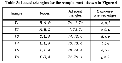
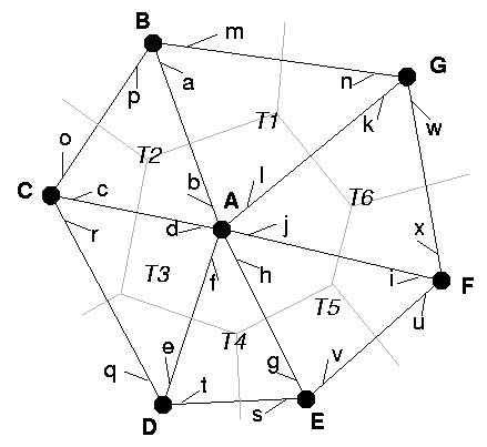
Figure 4: Sample mesh consisting of 7 nodes, 6 triangles, and 24 directed edges. Capital letters indicate nodes, numbers T1 etc denote triangles, and small letters indicate directed edges. Half-arrows pointing toward the destination node indicate the orientation of the directed edges.
Figure 5: Illustration of numbering of triangle nodes, adjacent triangles, and clockwise edges in Triangle data objects.
Figure 6: Illustration of steepest-descent flow routing in TIN framework.
Figure 7: Example of lake formation in the CHILD model. The green asterisks denote lake nodes. The lake has formed in response to a "digital dam" that was created by artificially raising the elevation of nodes near the catchment outlet. The lake outlet is indicated by the thick blue line at the right-hand edge.
Figure 8: Illustration of mass flux across the Voronoi polygon face between two adjacent nodes. Mass flux per unit contour width is calculated based on the gradient between A and B, and total flux is obtained by multiplying by the width of the shared Voronoi polygon edge.
Figure 9: Numerical solution to hillslope diffusion equation (eq 4) on a 5000-triangle TIN (inset), compared with an analytical solution. TIN represents a rectangular domain with two fixed boundaries. Open circules show nodes in the TIN viewed from the side. Solid line shows analytical solution in 1D. (Circles along x-axis are boundary points).
Figure 10: Numerical solution to simplified 2D groundwater flow equation (eq 5, substituting surface gradient for water surface gradient) on a straight hillslope (inset), compared with a 1D analytical solution. Symbols show nodes in the TIN viewed from the side. Solid line shows analytical solution in 1D.
Figure 11: Example landscape evolution simulation using the CHILD model.
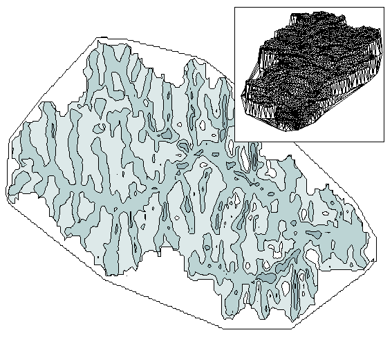
Figure 12: Contour plot showing simulated depth to water table under constant recharge, Forsyth Creek catchment, Fort Riley, Kansas, using the TRIBS model. Darker colors correspond to shallower water table. Inset shows catchment topography represented by TIN mesh.
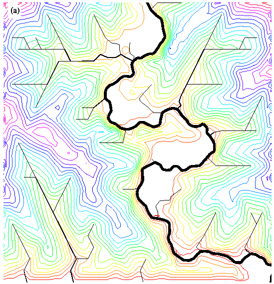
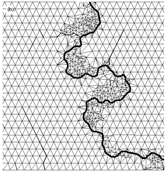
Figure 13: Simulation of 3D floodplain development by lateral stream migration (meandering). An adaptive meshing strategy is used to dynamically move, add, and delete points in response to lateral movement along the main channel. (a) Contour map of simulation. (b) Triangulation, showing densification of mesh in response to stream migration. Straight channel segments are artifacts of low mesh resolution outside of the meander belt.
 , (EQ 1)
5.1 One-dimensional network transport
Transport of water and sediment within drainage networks is often modeled as a quasi-one-dimensional problem, with the network essentially treated as a cascade of one-dimensional stream segments. In modeling landscape evolution, an equation for dynamic changes in surface elevation due to fluvial erosion or deposition can be written as
 , (EQ 2)
5.2 Two-dimensional diffusive transport
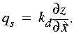
Diffusive transport processes typically require a fully two-dimensional solution and must therefore be handled in a different manner. Examples of such quasi-diffusive processes include groundwater flow, hillslope sediment transport, and lava flow. In modeling 2D mass transport on an irregular finite-difference mesh, the width of the interface between adjacent nodes must be known in order to compute the total mass exchange. Consider, for example, sediment transport by hillslope processes such as soil creep, which is commonly modeled as a linear (e.g., Culling, 1960) or nonlinear (e.g., Howard, 1994) function of surface gradient. In its linear form, sediment transport per unit contour width, qs, is given by
 , (EQ 3)
 , (EQ 4)
 , (EQ 5)
6. Examples
We have applied these data structures and algorithms in a simulation models of long-term landscape evolution (Tucker et al., 1997 and in prep.) and of catchment rainfall-runoff. Figure 11 shows a simulated drainage basin responding to a period of rapid baselevel lowering. Basin evolution is driven by a sequence of randomly generated storms, with fluvial erosion and sediment transport modeled on the basis of slope and total discharge at each point.
7. Summary and conclusions
We have presented a set of data structures and associated algorithms that facilitate TIN-based terrain modeling, with an emphasis on geologic and hydrologic applications. The framework is particularly well suited to applications involving dynamic changes in surface morphology and, more generally, to applications in which nodes (as opposed to triangles) are used as the basic computational elements. The data structure provides an efficient means of storing both a Delaunay triangulation and its corresponding Voronoi diagram. By using Voronoi polygons rather than triangles as the computational elements, the problem of distinguishing between flow within and between triangles is avoided. Voronoi polygons also provide a natural basis for solving diffusion-like equations numerically, using Voronoi polygon edges to approximation the effective contour width between each pair of adjacent nodes.
Acknowledgements
This work was supported by the U.S. Army Corps of Engineers Construction Engineering Research Center (DACA88-95-R-0020), by the Army Research Office (DAAH04-95-1-0181), and by the National Aeronautics and Space Administration. R.L.T.'s grandfather graciously pointed us toward relevant computational geometry literature.
References
Tables
Figures
Appendix A: Pseudo-code for Lake Fill algorithm
The Lake Fill algorithm uses a flag to indicate whether a node is a normal self-draining node (Unflooded), a pit for which an outlet has yet to be resolved (Pit), a flooded node that is part of the "lake" currently being computed (CurrentLake), or a flooded node that is part of a lake identified on a previous pass (Flooded). The algorithm assumes that initially all nodes have already been flagged as either Unflooded or Pit by the drainage direction finding routine.
ENDIFAppendix B: Algorithm for resolving flow directions within a closed depression
The algorithm shown below resolves drainage directions within a closed depression after an outlet point has been identified. The algorithm attempts to find the shortest path toward the outlet by iteratively scanning the neighbors of each node. A node is assigned to flow toward the closest of any neighbors whose drainage has already been resolved. The process continues until a drainage direction has been assigned to every node. The net effect of this procedure is that drainage is resolved sequentially in an "upstream" direction, starting from the depression's outlet.