Return to GeoComputation 99 Index
A.T. Murray
Australian Housing and Urban Research Institute, Department of Geographical Sciences and Planning, University of Queensland, Brisbane, Queensland 4072 Australia
S.R. Phinn
Department of Geographical Sciences and Planning, University of Queensland, Brisbane, Queensland 4072 Australia
Applications of cellular models to model landscape transformation processes have been undertaken by a number of researchers in the area of modeling urban and regional growth. In particular, Clark et al., (1997) have been successful in using CA to develop a model of the historical development of the San Francisco Bay and Washington D.C. areas. In this model the simple rules of CA are adapted to deal with probabilities of location by incorporating hard constraints, such as topography, road networks, and patterns of existing and historic settlement, that exclude or influence development. A particular feature of the model was its ability to self-modify related to thresholds associated with rapid growth or stagnation. The resulting simulations showed striking similarity with snapshots of historic development of the area.
The rapid development of spatial information technologies (primarily the development of Geographic Information Systems (GIS) and raster image processing and modeling tools) over the last few decades has allowed the space-time realization of many cellular models. The increasing availability of higher spatial resolution image data and the number of sources of remotely sensed imagery have provided a temporal information dimension from which time series analysis can provide stochastic representation of landscape transformations (Aplin et al. 1997). Cellular models in particular offer a useful space-time modeling environment in which raster-based information on spatial and temporal landscape change (derived from remotely sensed imagery) and information on factors that influence change (e.g., topographic factors derived from a digital elevation model) can be brought together. These types of models provide effective ways of understanding the process of urban development as well as offering a means of evaluating the environmental and social consequences of alternative planning scenarios.
In this paper, a cellular model of urban growth is developed. The conception and implementation of the model is orientated towards application of the model as a planning tool in which growth scenarios can be developed and evaluated, and 'what-if' type questions asked. Using contemporary software development tools the model is developed with a user friendly graphical interface and linked to a GIS that provides data for the model and analytic tools for evaluating model simulations. The first section of the paper gives a background and context for model development. A description of the conceptual development of the model is then given followed by a brief discussion on model implementation. To conclude, the spatial data requirements of the model are discussed, and the results of some preliminary simulation runs are presented.
In considering the context for the development of the model presented in this paper, emphasis was given to models dealing with the spatial configuration of urban form. Often born out of what has become known as social physics, numerous models of urban growth and development exist and have their origins in economic theory (e.g., Brotchie et al. 1980), size relationship between cities (Zipf, 1949), or are based on social and ethnic interactions. These models can be viewed as static and analytic, being able to explain urban expansion, but are limited in their ability to simulate urban development. Aggregated units such as political or administrative boundaries, census districts, or transport planning zones usually define the spatial characteristics of these models.
More recently there has been a trend towards cellular models that explains urban development in terms of principles of self-organisation where large-scale urban structure evolves from local scale decision making processes (Batty and Xie, 1994). In particular, computer models based on cellular automata (CA) are at the foundation of many of these models. The cellular model developed in this paper belongs to this class of models.
Cellular models of urban development that are based directly on classical CA, or are closely related to CA, have four main components. Firstly, the simulation process operates on lattice of cells in 2-dimensional space. A fundamental characteristic of the lattice is that cells have some adjacency or proximity to one another. Usually the lattice is a uniform gridded space, but potentially cells can be of any shape. Secondly, each cell in the lattice can adopt only one state of a set of possible states defined by the system being modeled. Thirdly, the configuration of the neighborhood of a cell defines the current state of the cell. In classical CA's, the neighborhood is usually the four or eight nearest neighbors. Fourthly, there is a set of transition rules that govern the types of changes in cell states in relation to the neighborhood configuration. For classical CA models, these rules are uniform across the lattice.
In the CA models of urban development, the strict application of a number of these components, such as uniform transition rules and the size of the neighborhood, have been relaxed. For urban systems it is unlikely that a local nearest neighbor neighborhood will be adequate to capture the spatial interactions necessary to produce a useful simulation. Batty and Xie (1994) present a cellular model that has the possibility of a nested set of neighborhoods and where the allocation of a birth depends on the inverse distance from the neighborhood's focal cell. Similarly, Semboloni (1997) uses a combination of an 8-cell neighborhood to check local density, and an extended neighborhood in which travel distance is accounted for to allocate a birth. White et al. (1997) used a 112-cell neighborhood to simulate the land-use pattern of Cincinnati, Ohio, arguing that a larger neighborhood allows a more realistic representation of the interaction among land uses.
In applying cellular models to urban development, transition rules must reflect significant factors that influence urban development and consequently can comprise a range of socio-economic and biophysical factors. Wu (1997) treats transition rules related to land use types as a fuzzy set, and only the transition rule with the highest grade of membership of the set is implemented as a change in cell state. Multiple cell states (residential, industry, and commercial) are modeled by White et al. (1997) using transition potentials on a neighborhood derived from calibration of the model using historic data on urban growth activities. Semboloni (1997) develops transition rules based on a land rent and demand model that considers white collar, blue collar, service, and base activities. Clarke et al. (1997) developed a model of historic urbanisation of the San Francisco Bay area in which transition rules are based on topography and distance from road networks, and are able to self-modify depending on growth rates.
Much of the work developing cellular urban models has been orientated towards either models that are designed for exploring the urban process as an artificial world (e.g., Cecchini, 1996, Portugali et al. 1997) or, more commonly, models that are calibrated with historic data and are used to project future growth patterns (e.g., Clarke et al. 1997). A limitation of models used for prediction, even if they are well calibrated, is that they have a tendency to predict urban sprawl. In an environment where a greater emphasis is placed on issues of sustainability in urban development, models that can simulate growth realistically but also be operated as an urban planning tool to build projected growth scenarios and answer 'what-if' type questions would be more valuable than predictive tools alone.
Data on urban population density ![]() , has been found to conform to the relation (Clark, 1951):
, has been found to conform to the relation (Clark, 1951):
![]()
where ![]() is the radial distance from the CBD,
is the radial distance from the CBD,![]() is the density gradient and
is the density gradient and ![]() is the central density. Urban models based on economic theory (Muth, 1969), discrete choice theory (Anas, 1982) and other approaches such as entropy-maximization (Wilson, 1970) have made widespread use of the negative exponential function. Braken et al. (1992) developed a model of urban growth in which logistic growth and Laplacian diffusion account for growth (births), and inhibitory effects associated with congested areas and migration modify growth and spread. In the model developed here, logistic growth and Laplacian diffusion are used to account for births in the form of a reaction-diffusion equation in which the birth rate is expressed as the rate of change of density with respect to time:
is the central density. Urban models based on economic theory (Muth, 1969), discrete choice theory (Anas, 1982) and other approaches such as entropy-maximization (Wilson, 1970) have made widespread use of the negative exponential function. Braken et al. (1992) developed a model of urban growth in which logistic growth and Laplacian diffusion account for growth (births), and inhibitory effects associated with congested areas and migration modify growth and spread. In the model developed here, logistic growth and Laplacian diffusion are used to account for births in the form of a reaction-diffusion equation in which the birth rate is expressed as the rate of change of density with respect to time:
where ![]() is an intrinsic growth rate,
is an intrinsic growth rate, ![]() is the carrying capacity, and
is the carrying capacity, and ![]() is the diffusion coefficient.
is the diffusion coefficient.
In our model, urban growth is considered to take place on a two-dimensional lattice of size ![]() , in which a cell state,
, in which a cell state, ![]() at any time
at any time ![]() can adopt two states developed or undeveloped. In the model, no account is taken of changes in internal urban structure in terms of deaths (change from developed to undeveloped) implying the model is a birth only type with no deaths. Future multi-state models could include a number of urban states such as residential, commercial, and industrial, with consideration of changes from one state to another over time.
can adopt two states developed or undeveloped. In the model, no account is taken of changes in internal urban structure in terms of deaths (change from developed to undeveloped) implying the model is a birth only type with no deaths. Future multi-state models could include a number of urban states such as residential, commercial, and industrial, with consideration of changes from one state to another over time.
To begin the simulation process, births ![]() are generated using the solution to equation (2) expressed as an occupation probability
are generated using the solution to equation (2) expressed as an occupation probability ![]() , calculated as
, calculated as ![]() . Under steady state conditions, equation (2) can be solved on a lattice by using a finite difference scheme that repeatedly averages the neighbors of a cell
. Under steady state conditions, equation (2) can be solved on a lattice by using a finite difference scheme that repeatedly averages the neighbors of a cell ![]() , over a neighborhood space
, over a neighborhood space ![]() , of size
, of size ![]() (measured in cells), using weights to account for neighbor proximity (Rucker and Walker, 1997). To generate births, a neighborhood
(measured in cells), using weights to account for neighbor proximity (Rucker and Walker, 1997). To generate births, a neighborhood ![]() at any time
at any time ![]() , receives births at time
, receives births at time ![]() , if the occupation probability
, if the occupation probability ![]() is greater than the current neighborhood occupation proportion. This is expressed as
is greater than the current neighborhood occupation proportion. This is expressed as
where ![]() . If
. If ![]() = 1, the number of births
= 1, the number of births ![]() , deemed to occur is then calculated as
, deemed to occur is then calculated as
![]()
A location for a birth at a cell![]() ,
, ![]() is then chosen by conceptualising the neighborhood space
is then chosen by conceptualising the neighborhood space ![]() to represent an infrastructure grid for service provision. Since services such as power and water are usually derived from and developed network, the probability
to represent an infrastructure grid for service provision. Since services such as power and water are usually derived from and developed network, the probability ![]() of a cell being developed decreases with distance from developed cell.
of a cell being developed decreases with distance from developed cell. ![]() . The spatial implication of this is that development units are correlated in space (Makse et al. 1995). This can be expressed as an inverse power law where
. The spatial implication of this is that development units are correlated in space (Makse et al. 1995). This can be expressed as an inverse power law where ![]() is distance from cell
is distance from cell ![]() and
and ![]() is a tunable distance parameter:
is a tunable distance parameter:
The location ![]() , of each of the
, of each of the ![]() births at some cell
births at some cell ![]() , in neighborhood space
, in neighborhood space ![]() is then determined such that there is no directional bias in the location of cell
is then determined such that there is no directional bias in the location of cell ![]() in
in ![]() (Batty, 1997), and is calculated as:
(Batty, 1997), and is calculated as:
where ![]() is a random normal variable between 0 and 1. To complete the simulation of the neutral model, the state of cell
is a random normal variable between 0 and 1. To complete the simulation of the neutral model, the state of cell ![]() at time
at time ![]() is calculated as
is calculated as
![]() .
.
Simulations using the neutral model produced morphologies shown in Figures 1a and1b. Figure 1a shows the distribution of developed cells according to the negative exponential function given by equation (1) in which a city grows on an ideal surface on which there are no influences or impediments to growth. Figure 1b shows the distribution of developed cells for which the infrastructure grid was implemented to allocate births. The distribution of cells is much more 'clumped,' as is true of real cities, where urban development attracts further development.
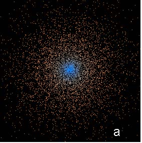
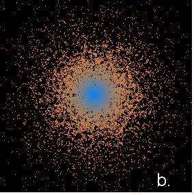
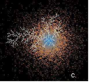
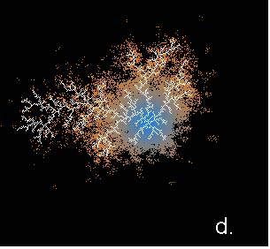
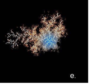
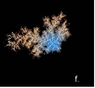
Figure 1. a) Results of a simulation using the neutral model showing simple negative exponential growth in which there are no influences or impediments to growth. b) negative exponential growth with implementation of the infrastructure grid causing 'clumping' of development units. c) an artificial transport network generated using a process of Diffusion Limited Aggregation superimposed on figure b. d,e,f) results of a simulation imposing increasing constraint on growth associated with distance the artificial transport network.
The growth of cities is influenced strongly by socio-economic and biophysical constraints, and institutional controls. Physical factors such as water bodies and steep terrain constrain growth as do institutional controls that prohibit growth. Economic factors such as distance from transport networks, distance from commercial outlets and land values also play a significant role. To demonstrate the influence of constraints on the distribution of developed cells shown in Figure 1b., an artificial constraint surface similar to a transport network was introduced into the simulations. This network, shown in Figure 1c., superimposed on Figure 1b, was developed using a process of Diffusion Limited Aggregation (DLA) (Batty,1991). Distance from the network to any cell ![]() on the lattice is treated as a probability such that the further a cell is from the transport network the less likely the cell will be developed. The results from simulations using the constraints network are shown in Figures 1d to 1f.
on the lattice is treated as a probability such that the further a cell is from the transport network the less likely the cell will be developed. The results from simulations using the constraints network are shown in Figures 1d to 1f.
Figures 1d to 1f depict spatial distributions closely related to the extent of the artificial transport network. The distributions have a dense inner core (like a CBD) with the distribution of developed cells declining with distance from the dense inner core. There is a tendency for developed cells to aggregate at branching points along the network as is often the case when commercial centers develop at the junction of major roads in cities. There also are aggregated groups of developed cells that are unattached to the dominant core of developed cells, as typically occurs on the fringes of cities.
To incorporate these ideas into a model of a real city in which economic and physical factors play a significant role in the location of developed cells, we introduced a constraint vector ![]() of
of ![]() constraints into the model. In the model
constraints into the model. In the model ![]() has three elements (
has three elements (![]() ) associated with: 1) institutional controls, 2) physical constraints, and 3) geographic constraints. Institutional controls
) associated with: 1) institutional controls, 2) physical constraints, and 3) geographic constraints. Institutional controls ![]() resulting from land tenure and planning policies can be represented in binary form, that is
resulting from land tenure and planning policies can be represented in binary form, that is ![]() such that
such that ![]() if development can occur, or
if development can occur, or ![]() if development is prohibited. Similarly, physical constraints
if development is prohibited. Similarly, physical constraints ![]() result from physical barriers to development such as water bodies and flood zones. Geographic constraints
result from physical barriers to development such as water bodies and flood zones. Geographic constraints ![]() are associated with economic and physical factors that do not necessarily prohibit growth but act to modify growth patterns. Other factors that influence growth could also be introduced into the model but for the purposes of this model the constraint vector is given by:
are associated with economic and physical factors that do not necessarily prohibit growth but act to modify growth patterns. Other factors that influence growth could also be introduced into the model but for the purposes of this model the constraint vector is given by:
In our model we consider three geographic constraints: land slope ![]() , distance from road
, distance from road ![]() , and distance from population centers
, and distance from population centers ![]() . The assumption here is that these geographic constraints modify growth patterns according to some function of their magnitude. For example, as growth occurs on the urban fringe, the likelihood of development taking place decreases as slope, and distance from transport network increase. The geographic constraint variables are represented on a lattice with cell size equivalent to the neutral model and each cell
. The assumption here is that these geographic constraints modify growth patterns according to some function of their magnitude. For example, as growth occurs on the urban fringe, the likelihood of development taking place decreases as slope, and distance from transport network increase. The geographic constraint variables are represented on a lattice with cell size equivalent to the neutral model and each cell ![]() is calculated to have a geographic constraint probability
is calculated to have a geographic constraint probability ![]() given by:
given by:
where ![]() represents the probability of the
represents the probability of the ![]() geographic constraint at cell
geographic constraint at cell ![]() , and
, and ![]() is a weight that specifies the relative importance of the
is a weight that specifies the relative importance of the ![]() geographic constraint. The probability
geographic constraint. The probability ![]() , is calculated using a nonlinear function of the form:
, is calculated using a nonlinear function of the form:
where ![]() is a dummy variable representing the
is a dummy variable representing the ![]() geographic constraint and
geographic constraint and ![]() is a tunable parameter.
is a tunable parameter. ![]() is then determined as:
is then determined as:
Using the neutral model given by equation (5) in which a birth is generated and located, the geographic model is completed with the inclusion of the constraint vector ![]() to give:
to give:
 .
.
![]()
The hypothesis that the model behaves like a stochastic spatial optimization process requires testing in a number of different areas. First, what is the model optimizing for? The model requires boundary conditions that can be derived from population projections. For example, if a planning scenario allocates a certain population growth to an area, a simulation can be run until the area allocated to development by the simulation is the same as the area required by the projected population growth. In the model, constraint variables are associated with the cost of distance from particular desirable urban facilities such as commercial centers and transport networks. Given initial conditions (urban extent) and boundary conditions (projected growth) the model can be seen to be optimally allocating development units with respect to distance from facilities. Given that travel distance plays an important role in the economic (e.g., distance from facilities) and environmental (e.g., energy use, air pollution) well being of a city, the model could be applied to addressing sustainability issues in growing urban regions.
Second, questions associated with the way the model works at different scales needs to be addressed. The model stochastically allocates development units on a local development unit basis (a cell). It can be argued that the model optimizes the location of each development unit in its local neighborhood; however, does this lead to a global optima for a particular growth scenario? This question could be answered by comparing a linear programming optimization to the same growth scenario as is simulated by the model. Further work is required to validate the model presented in this paper as an stochastic spatial optimization approach.
The model outlined in the previous section provides a method for exploring the spatially optimal allocation of development units in the landscape. Tunable parameters and weights in the model offer a means of exploring different development scenarios. By modifying constraint information, 'what-if' type questions can be asked of the model, and spatially optimal results developed.
The approach to implementing the model is to view it as a potential urban planning tool that could be used by planners and local governments to explore growth scenarios associated with population projections. So as to make the model as user friendly as possible, advantage is taken of contemporary software development tools and Geographic Information System (GIS) tools. Software development tools allow development of friendly graphical users interfaces (GUI). In particular, DELPHI (object orientated pascal) is used to implement the mathematical model and develop the GUI. To apply the model, the constraint vector requires information on institutional controls, physical constraints, and geographic constraints. Since the model operates on a lattice, raster data is required to produce spatial output. To meet the data requirements of the model, the model and GUI are linked to a GIS, (ArcView Spatial Analyst), which stores and manages raster data sets.
Software design comprises a main menu and a series of pull down sub-menus that initiate data input and output, parameter setting, data viewing, and model choices. Data transfer between the modeling software and the GIS is via binary data files. Before running the model, data are loaded from the GIS and parameters are set according to the scenario being explored. Neighborhood parameters are the neighborhood size ![]() and distance parameter
and distance parameter ![]() . Each variable geographic constraint
. Each variable geographic constraint ![]() has a tunable parameter
has a tunable parameter ![]() that can be varied using slider bar controls. Information on institutional controls
that can be varied using slider bar controls. Information on institutional controls ![]() associated with planning policies can be modified in the GIS before inputting to the model. Model simulations can be viewed in real time using DELPHI graphics and the results of simulation runs read as binary files by the GIS and displayed with overlay of contextual data stored in the GIS.
associated with planning policies can be modified in the GIS before inputting to the model. Model simulations can be viewed in real time using DELPHI graphics and the results of simulation runs read as binary files by the GIS and displayed with overlay of contextual data stored in the GIS.
Data on institutional controls ![]() is derived from a Digital Cadasta Database for the region. For this exercise tenure was used to identify areas for which development can proceed or be excluded. The assumption is that all non-developed freehold land is available for development, while state owned land, such as reserves and state forests is unavailable. Data on physical constraints
is derived from a Digital Cadasta Database for the region. For this exercise tenure was used to identify areas for which development can proceed or be excluded. The assumption is that all non-developed freehold land is available for development, while state owned land, such as reserves and state forests is unavailable. Data on physical constraints ![]() , such as water bodies, is derived from the 1988 and 1995 image classification maps. No information of flood zones is used in the model at this stage and this is a limitation because large areas of the low-lying coastal plain of the Gold Coast are subject to flooding that prohibits urban development.
, such as water bodies, is derived from the 1988 and 1995 image classification maps. No information of flood zones is used in the model at this stage and this is a limitation because large areas of the low-lying coastal plain of the Gold Coast are subject to flooding that prohibits urban development.
Three geographic constraint variables: land slope, distance from major and minor road networks, and distance from major commercial centers are used in the simulation runs presented here. Land slope was derived from a Digital Elevation Model of the area (with 50m resolution), using the slope derivation procedure available in ArcView Spatial Analyst. A Euclidean distance function in ArcView Spatial Analyst computed the distance from major and minor road networks and from major commercial centers.
The GIS was used as a spatial database in the simulation process to provide data storage, manipulation and display functionality for both the model and ancillary data. It is likely in application that many simulation runs will be performed and the results of simulation runs explored and evaluated. The results of the simulation runs can be imported as spatial layers into the database and contextual information (e.g., census data) and analytical GIS tools applied to evaluate different growth scenarios.
Figure 2. a.) Actual urban growth from 1988 to 1995 for the Gold Coast area. b.) Simulated urban growth for the Gold Coast area.
In the actual growth shown in Figure 2a. there is a substantial amount of in-filling (i.e., growth within the existing urban matrix), and this type of growth also is produced by the model. A large amount of the actual growth for the Gold Coast has occurred around the major highway that runs parallel to the coast, east of the urban area. While the simulation shows road influenced growth, it tends to be more dispersed than the actual growth, which in some areas occurs in large development blocks. The simulation underestimates the extent of growth north of the region, and this can be attributed to the absence of a commercial center in this area that is used in the simulation run. When the constraint on distance from commercial centers is relaxed, the model places a large amount of development in this area. It is of note that the local government authority that controls growth on the Gold Coast is planning a large amount of development in this area. As yet, no information on flood zones has been used in simulation runs and the model will have a strong tendency to place development on these areas as they are usually prime areas for development if no limitation due to flooding existed.
The possibility of the application of the model as method of optimization would give simulations more value in a planning environment. To validate the model as an optimization method requires comparison with other existing methods of optimization. In particular, the issue of whether the model produces a globally optimal result in a spatial context needs addressing. If it is found that the local allocation of development units by the model leads to a spatially global optimization it has the advantage over existing optimization approaches that tend to use aggregated land units. Work could be carried out to make formal mathematical links with existing optimization approaches used in urban decision support systems.
The issue of constraint parameter estimation is an important one. The model can potentially simulate a wide variety of urban forms depending on parameter values associated with the constraint variables. Currently parameter estimates are developed using visual calibration (Clarke et al. 1997, White et al. 1997). Parameter estimates could be derived by developing statistical relationships between the information on urban extent and the constraint variables used in the model. For example, using information on urban extent and change over time derived from remotely sensed data, logistic regression techniques could be applied to develop relationships with the constraint variables (e.g. slope, distance from commercial centers) that allow parameter estimates to be made.
Anas, A., 1982. "Residential Location Markets and Urban Transportation: Economic Theory, Econometrics and Policy Analysis with Discrete Choice Models," Academic Press, New York, NY.
Aplin, P., P. Atkinson and P. Curran, 1997. "Fine spatial resolution satellite sensors for the next decade," International Journal of Remote Sensing, 18(18): pp. 3,873-3,881.
Batty, M., 1991. "Generating Urban Forms from Diffusive Growth," Environment and Planning A, 23: pp. 511-544.
Batty, M. and Y. Xie, 1994. "From Cells to Cities" Environment and Planning B, 21: pp. 531-548.
Batty, M. and Y. Xie, 1997. "Possible Urban Automata," Environment and Planning B, 24: pp. 175-192.
Bracken, A.J. and H.C. Tuckwell, 1992. " Simple Mathematical Models for Urban Growth," Proceedings of the Royal Society of London, 438: pp. 171-181.
Brotchie, J., J. Dickley and R. Sharpe, 1980. "TOPAZ-General Planning Technique and its Application at the Regional , Urban, and Facility Planning Level," Springer-Verlag, Berlin, Germany.
Cechini, A., 1996. "Urban Modelling by Means of Cellular Automata: Generalised Urban Automata with the Help On-Line (AUGH) model," Environment and Planning B, 23: pp. 721-732.
Clarke, K.C., S. Hoppen and L. Gaydos, 1997. "A Self-Modifying Cellular Automaton of Historical Urbanization in the San Francisco Bay Area," Environment and Planning B, 24: pp. 247-261.
Makse, H.A., S. Havlin and H.E. Stanley, 1995. "Modelling Urban Growth Patterns," Nature, 3: pp. 608-612.
Muth, R., 1969. "Cities and Housing: The Spatial Pattern of Urban Residential Land Use," Chicago University Press, Chicago, IL.
Portugali, J., I. Benenson and I. Omer, 1997. "Spatial Cognitive Dissonance and Sociospatial Emergence in a Self-Organizing City," Environment and Planning B, 24: pp. 263-285.
Semboloni, F., 1997. "An Urban and Regional Model Based on Cellular Automata", Environment and Planning B, 24: pp. 589-612.
Ward, D.P., A.T. Murray and S.R. Phinn, 1999. "Monitoring Growth in Rapidly Urbanising Areas Using Remotely Sensed Data," The Professional Geographer, [in review].
White, R., G. Engelen and I. Uljee, 1997. "The Use of Constrained Cellular Automata for High-Resolution Modelling of Urban Land-Use Dynamics," Environment and Planning B, 25: pp. 323-343.
Wilson, A.G., 1970. "Entropy in Urban and Regional Modelling," Pion Press, London, England.
Wu, F., 1996. "A Linguistic Cellular Automata Simulation Approach for Sustainable Land Development in a Fast Growing Region," Computers, Environment and Urban Systems, 20: pp. 367-387.
Zipf, G.K., 1994. "Human Behaviour and the Principles of Least Effort," Addison-Wesley Publishing Company, Cambridge, MA.