
 |
Return to GeoComputation 99 Index
Robert J. Abrahart
School of Earth and Environmental Sciences, University of Greenwich, U.K.
E-mail: bob@ashville.demon.co.uk
Linda See and Pauline E. Kneale
School of Geography, University of Leeds, U.K.
E-mail: l.see@geog.leeds.ac.uk | pauline@geog.leeds.ac.uk
Software tools can now be used to translate neural network solutions into standard computer languages and source code. This conversion process enables trained networks to be implemented as embedded functions within existing hydrological models or assembled into standalone computer programs. In addition to their normal use, embedded functions can provide new opportunities for dynamic testing, and for internal investigation of the modelling function through saliency analysis i.e., disaggregation of a neural network solution in terms of its forecasting inputs. Example time series visualizations of saliency analysis applied to three neural network hydrological forecasting models are presented and discussed.
This paper examines the performance of neural network solutions when the input data are omitted on a systematic basis during a series of simulation modelling experiments. Examples are then provided to illustrate the process of neural network disaggregation. This disaggregation process, termed saliency analysis, is based on a neurocomputing method for assessing the relative importance of internal components and offers some potential to generate useful information on the processes and relationships involved. It can, for example, be used to examine the direction and magnitude of various individual relationships through the act of excluding one or more variables, and explore inherent variations associated with the remainder. Neural networks are ideal tools for this type of analysis due to the distributed nature of their information processing structure, which enables different inputs to be omitted while the model is running. Three neural network hydrological modelling solutions (Abrahart et al., 1998) are examined using single input saliency analysis. Each neural network was designed to produce a continuous series of one-step-ahead river flow predictions based on hydrological and meteorological inputs for the Upper River Wye in Central Wales. To facilitate the input saliency analysis operation each network was converted into an embedded function. Time series plots revealed that different inputs influenced different aspects of the forecast hydrograph, which could have some significance for understanding hydrological processes, although further evaluation is required to confirm the nature and extent of this approach.
To gain understanding from a computer model one must first acquire and decipher evidence about the nature of the modelling processes that occur within the software program. But a multilayered neural network solution, with its preponderance of local processing operations and weighted relationships, is often too complex, or too demanding, for direct intelligible comprehension, e.g. Abrahart et al. (1998) employed a standard neural network architecture that had 22 inputs, 30 hidden units, and 590 weighted connections. For networks without hidden layers, the strength of internal relationships can be determined from direct examination of the connection weights (Tang et al., 1991; Maier & Dandy, 1996a). Some software packages also provide tools that can be used for analysing the pattern of weights; a common example is the Hinton Diagram. This instrument uses squares of different sizes or colours to provide a graphical representation of the weighted connections (Bishop, 1995: p120; SNNS Group, 1995: p53). Examining individual weighs is a time consuming task and with large or complex multi-layered networks is not that rewarding. Interaction between the different components is important and with complex structures the exact strength and manner of influence associated with each particular item becomes more difficult to interpret. Traditional model building has a diagnostic procedure, termed sensitivity analysis, which investigates "the rate of change in one factor with respect to change in another" (McCuen, 1973). This method of assessment uses positive and negative manipulation of individual inputs to examine the effect of such alterations on the model output, which is quantified using global statistics. Sensitivity analysis can be applied to both traditional and neural models alike. Moreover, when compared to a detailed examination of weights, it has distinct advantages for investigating neural network solutions that have more than one hidden layer (Maier & Dandy, 1996b). But this technique is subject to potential drawbacks arising from improper combinations or actualisations. Some software packages also contain tools that can be used to compute a 2.5-D visualization of the relationship between two input vectors and either a hidden unit, or an output unit, to provide additional information. This is termed projection analysis (SNNS Group, 1995: p54). These various methods of analysis are the standard approaches that can be used to examine a neural network solution. Each existing technique has its merits, but such tools are of limited scope and application, and for complex solutions have insufficient capabilities to enable a purposeful or meaningful evaluation.
It is important to recognise that a major difference exists between neurocomputing solutions and standard equation-based tools--which still awaits detailed exploitation. Each neural network solution is a distributed information processing structure. The information that is needed to perform data processing operations is stored within the individual processing units and the weighted connections that exist between them. Each component within the overall structure is responsible for one small part of the total input-output mapping operation. This means that each individual data input can have no more than a marginal influence with respect to the complete solution. Each network or model will possess substantial fault tolerant characteristics. The mechanism will still function, to generate reasonable mappings, in response to incomplete data or from data that contain noise and fuzziness; however, distributed information processing and the power to function with missing data also are important with respect to acquiring information on the model. The distributed nature of each device means that a network can be disaggregated in terms of its forecasting inputs and will still generate predictions, and the purposeful introduction of missing inputs can be used to provide relevant information on the internal processes. This disaggregation technique, saliency analysis, is derived from a need to assess the relative importance of different neural network components in terms of the effect that each item has on the error function. The removal or zeroing of input vectors in a similar manner will facilitate an examination of the relative magnitude and significance of internal relationships on predicted output, and this type of analysis can be performed in an operational context while the model is running. The direct consequence of each input vector within the overall structure is thus established through the effect that each missing item has on the error function, with respect to other input vectors under natural (as opposed to manufactured) conditions. The omission of inputs in a practical sense could involve setting the weights to zero, setting all node output values to zero, or passing zero values to the nodes. It must be stressed that saliency analysis is not a form of sensitivity analysis since the aim is not to examine "the rate of change in one factor with respect to change in another." It is a powerful tool that involves complete removal of individual items and piecemeal disaggregation of the modelling solution. Most standard neural network packages do not contain the tools that are needed to perform these types of operation on an iterative or interactive basis so alternative implementation strategies are therefore required.
Several neural network simulation packages will translate a standard back-propagation solution into Third Generation Language (3GL) computer code such as C or Pascal. The output from this conversion process can be operated as an embedded function using standard program calls, either within a bespoke program, or coupled to an existing model, as an integrated part of the larger whole, e.g., in a hybrid simulation model of transient water flow within branched water pipeline systems (Van den Boogaard & Kruisbrink, 1996). But the general concept of using embedded neural network functions also can be made to work in reverse. Simple programs can be used to evaluate individual neural network solutions or to extend their modelling capabilities into areas or scenarios that exceed the confines of the original task that the network was intended for or was trained to accomplish. Abrahart (1998), for example, used this approach to examine the impact of accumulated error on a one-step-ahead neural network hydrological modelling solution. The network input data were manipulated using a combination of external feedback loops and simple column swapping routines to facilitate prediction-based updates. The end result of this operation was at each time step passed to an embedded neural network function for processing. This combined mechanism was used to investigate the power of neural network solutions to perform temporal modelling over various periods of time without the benefit of river flow updates. In addition to providing greater periods of forward prediction, the implementation was used to assess the original solution in terms of extended predictive capabilities, and in terms of progressive degradation associated with accumulated error over time.
In this example embedded functions were used to perform an input saliency analysis operation, which involved zeroing one input data stream at a time, with subsequent replacement after each computation. Three neural network modelling solutions were examined. Full particulars on the construction and selection of each model are provided in Abrahart et al. (1998). Each neuro-forecasting application was a one-step-ahead prediction of river flow records for the Upper River Wye in Central Wales. Previous hydrological modelling of this catchment includes: Beven et al. (1984), Bathurst (1986) and Quinn & Beven (1993). Data for the Cefn Brwyn gauging station (No. 55008) comprised: rainfall (RAIN), potential evapotranspiration (PET), and river flow ordinates (FLOW) on a one-hour time step. To this list was added annual hour count (CLOCK). The input data (independent variables) corresponded to: sin (CLOCK), cos (CLOCK), RAIN t, RAIN t-1 to t-6, PET t, PET t-1 to t-6, FLOW t-1 to t-6. The output (dependent variable) was FLOW t in normalised [0-1] flow units (nfu). SNNS (Stuttgart Neural Network Simulator) was used to perform the modelling operations based on enhanced back propagation and a 22:16:14:1 architecture. The initial network was first trained on one annual data set and then tested with the other two. This operation was repeated for each annual data set and an optimal solution, for each model building scenario, selected. Data were taken from 1984, a drought year, 1985, that had a limited number of intermediate events, and 1986, a year with major floods.
The 'snns2c' software tool was used to convert the three trained networks into three individual C functions. These functions were called from a main program and computed:
Each annual data set was passed through each function and nine sets of annual output data computed, comprising one set per model, per annum. The numerical results were then examined.
Figures 1-4 plot time series for three 500-hour periods to illustrate aspects of the analysis. Each hydrograph contains predictions derived from input for one annual data period using a model that was developed on another. To facilitate visual interpretation each period has been plotted as four separate graphs to illustrate the variation associated with: CLOCK, RAIN, PET and FLOW. Likewise, common background colours are assigned to the different periods of time, and a log scale has been implemented to provide increased differentiation at low and intermediate levels of river flow prediction.
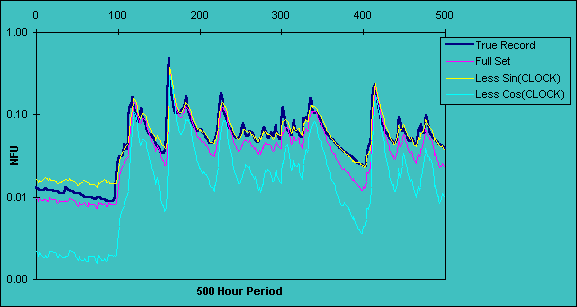
Figure 1a: Saliency analysis of model built with 1984 data for 500-hour period
08.00 : 25 March - 04.00 : 15 April 1985. Looking at the relative influence of each CLOCK input.
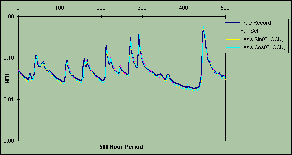
Figure 1b: Saliency analysis of model built with 1985 data for 500-hour period
14.00 : 6 December - 10.00 : 26 December 1986. Looking at the relative influence of each CLOCK input.
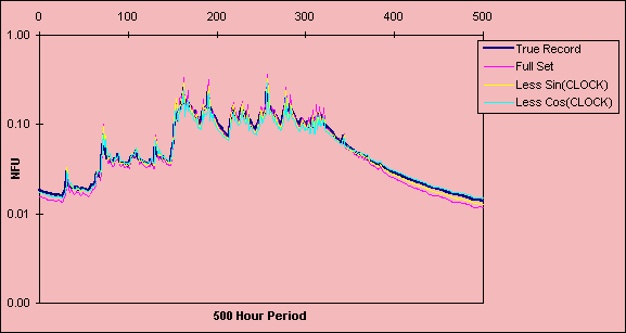
Figure 1c: Saliency analysis of model built with 1986 data for 500-hour period
00.00 : 26 January - 20.00 : 14 February 1984. Looking at the relative influence of each CLOCK input.
Figures 1a-c illustrate the effect of omitting the sine and cosine components of the CLOCK input, where the sine represents spring-autumn differences, and the cosine, the differences between winter and summer. The 1984 model was the only one in which the omission of either input caused major changes in the predicted output (Figure 1a). Omitting the cosine resulted in underpredictions while excluding the sine produced a more accurate prediction. This suggests that seasonal differences between the summer and winter were important for 1984 and that the cosine was an important input for allowing the network to differentiate between the summer drought period and regular winter flows. The negligible effects on the predictions from the 1985 and 1986 models implies that the seasonal differences were less important.
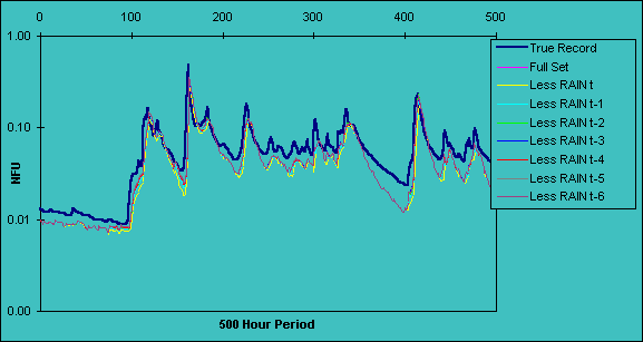
Figure 2a: Saliency analysis of model built with 1984 data for 500-hour period
08.00 : 25 March - 04.00 : 15 April 1985. Looking at the relative influence of each RAIN input.
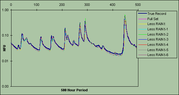
Figure 2b: Saliency analysis of model built with 1985 data for 500-hour period
14.00 : 6 December - 10.00 : 26 December 1986. Looking at the relative influence of each RAIN input.
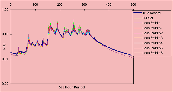
Figure 2c: Saliency analysis of model built with 1986 data for 500-hour period
00.00 : 26 January - 20.00 : 14 February 1984. Looking at the relative influence of each RAIN input.
The effects of excluding RAIN at t and t-x are provided in Figures 2a-c. The main result is the underprediction of flow prior to a late starting rise in the hydrograph, which is understandable given that rainfall is the driving force behind sharp increases in river level. The effect is most noticeable for the 1984 model tested with 1985 data (Figure 2a) since the model has been trained with data from a drought year and tested using data from a year with higher flows. Peak flow prediction does not appear to be affected.
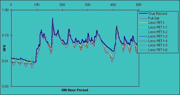
Figure 3a: Saliency analysis of model built with 1984 data for 500-hour period
08.00 : 25 March - 04.00 : 15 April 1985. Looking at the relative influence of each PET input.
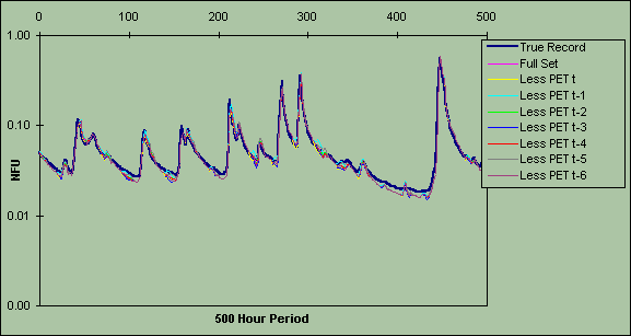
Figure 3b: Saliency analysis of model built with 1985 data for 500-hour period
14.00 : 6 December - 10.00 : 26 December 1986. Looking at the relative influence of each PET input.
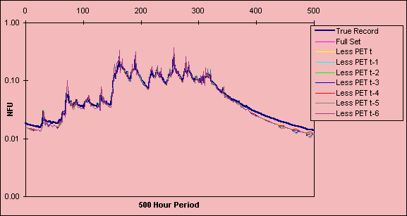
Figure 3c: Saliency analysis of model built with 1986 data for 500-hour period
00.00 : 26 January - 20.00 : 14 February 1984. Looking at the relative influence of each PET input.
Figures 3a-c demonstrate the result of omitting PET at t and t-x. Excluding this variable appears to affect low flows, which produced oscillations in the flow predictions; however, this is an artifact of plotting on a log scale and in practice the variation is negligible. In essence this shows that PET has a minimal impact on flows at this scale.
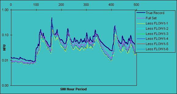
Figure 4a: Saliency analysis of a model built with 1984 data for 500-hour period
08.00 : 25 March - 04.00 : 15 April 1985. Looking at the relative influence of each FLOW input.
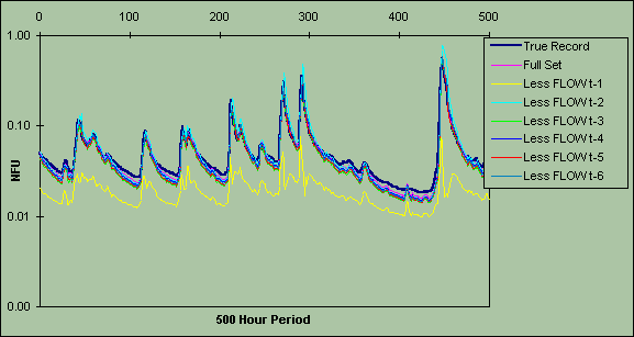
Figure 4b: Saliency analysis of model built with 1985 data for 500-hour period
14.00 : 6 December - 10.00 : 26 December 1986. Looking at the relative influence of each FLOW input.
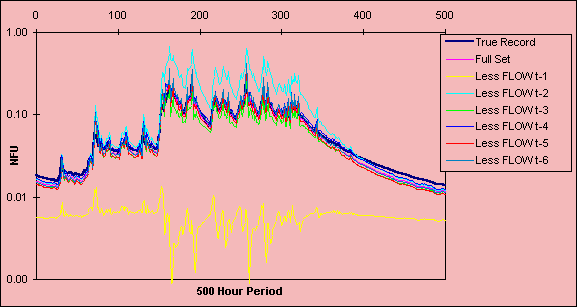
Figure 4c: Saliency analysis of model built with 1986 data for 500-hour period
00.00 : 26 January - 20.00 : 14 February 1984. Looking at the relative influence of each FLOW input.
The influence of omitting FLOW at t-x is provided in Figures 4a-c. FLOW at t-1 is clearly the most important factor as the omission of this variable produces lower predictions throughout, especially for 1986 (Figure 4c). The effect of omitting the other FLOW inputs has a similar, but smaller influence, although omission of FLOW at t-2 did produce some noticeable increases in peak flow prediction. Some degree of mutual interaction is therefore occurring between the past FLOW inputs at lags t-1 and t-2. This result concurs with an ARMA modelling solution that was fitted to the data, in which the second lag also was important (See et al., 1998).
Overall, saliency analysis has revealed that the two most important factors were FLOW at t-1 and t-2, although RAIN at t and t-x and the seasonal inputs had an influence on certain aspects of the hydrograph. The model developed on 1984 data required the seasonal correction factor, whereas the other two models were more dependent on previous FLOW records, with both conditions being a direct reflection of differing environmental circumstances and associated catchment response.
Modelling is a complex issue. The decision to use a neural network model should be made on the basis of employing the right tool for the appropriate task. The advantages associated with different types of solutions must be examined, which should include an investigation into the potential role and benefits associated with a neural network application. In addition to performing a basic mapping operation, the use of embedded functions offers untapped opportunities for increasing the role of neural network solutions; saliency analysis is just one item from a list of potential implementations.
Arguments against using neural networks are frequently based on the premise that they are nothing more than black box models that provide no scientific explanation or theoretical understanding of the fundamental processes. Both traditional models and neural networks are useful forecasting tools. Both can be used as test-bed structures to examine theories or explanations and can be employed to quantify dynamic relationships. The advantage of neural network simulation with saliency analysis as shown here is to permit the exploration of forecasts and the exploration of 'what-if' scenarios.
The flexibility of saliency analysis offers new opportunities to design and test models and to gain insights into the behaviour of a black box neural network approach. These explorations have demonstrated that saliency analysis is a useful tool and can be used to provide knowledge about internal relationships within a neural network architecture in terms of:
Moreover, saliency analysis can be used to assist at the development stage to:
This initial investigation was based on single input analysis of three different networks. The next step is to experiment with multiple input omission and explore the forecasting power associated with different combinations of input data. Like all modelling solutions, neural networks can be examined to provide some level of understanding, depending upon the method of investigation. The use of embedded function implementations is a new area of research that still requires further exploration.
Abrahart, R.J., 1998. "Neural networks and the problem of accumulated error: an embedded solution that offers new opportunities for modelling and testing." In: Babovic, V. and Larsen, C.L., Eds. 1998. Hydroinformatics '98: Proceedings Third International Conference on Hydroinformatics, Copenhagen, Denmark, 24-26 August 1998. Vol. 2. Rotterdam: A.A. Balkema, pp. 725-731.
Abrahart, R.J., L. See, and P.E. Kneale, 1998. "New tools for neurohydrologists: using 'network pruning' and 'model breeding' algorithms to discover optimum inputs and architectures." GeoComputation '98: Proceedings Third International Conference on GeoComputation, University of Bristol, 17-19 September 1998. Manchester: GeoComputation CD-ROM. ISBN 0-9533477-0-2.
Bathurst, J. 1986. "Sensitivity analysis of the Systeme Hydrologique Europeen for an upland catchment," Journal of Hydrology, 87, pp. 103-123.
Beven, K.J., M.J. Kirkby, N. Schofield, and A.F. Tagg, 1984. "Testing a physically-based flood forecasting model (TOPMODEL) for three U.K. catchments," Journal of Hydrology, 69, pp. 119-143.
Bishop, C.M. 1995. Neural Networks for Pattern Recognition. Oxford: Clarendon Press.
Maier, H.R. and G.C. Dandy, 1996a "Neural network models for forecasting univariate time series," Neural Network World, 5, pp. 747-772.
Maier, H.R. and G.C. Dandy, 1996b. "The use of artificial neural networks for the prediction of water quality parameters," Water Resources Research, 32, pp.1,013-1,022.
McCuen, R.H. 1973. "The role of sensitivity analysis in hydrologic modelling," Journal of Hydrology, 18, pp. 37-53.
Quinn, P. F. and K.J. Beven, 1993. "Spatial and temporal predictions of soil moisture dynamics, runoff, variable source areas and evapotranspiration for Plynlimon, Mid-Wales," Hydrological Processes, 7, pp. 425-448.
See, L., R.J. Abrahart, and S. Openshaw, 1998. "An integrated neuro-fuzzy-statistical approach to hydrological modelling." GeoComputation '98: Proceedings Third International Conference on GeoComputation, University of Bristol, 17-19 September 1998. Manchester: GeoComputation CD-ROM. ISBN 0-9533477-0-2.
SNNS Group, 1995. SNNS - Stuttgart Neural Network Simulator, User Manual, Version 4.1. Institute for Parallel and Distributed High Performance Systems, University of Stuttgart, Germany. Report No. 6/95.
Tang, Z., C. deAlmedia, and P.A. Fishwick, 1991. "Times series forecasting using neural networks vs. Box-Jenkins methodology," Simulation, 57, pp. 303-310.
Van den Boogaard, H.F.P. and A.C.H. Kruisbrink, 1996. "Hybrid modelling by integrating neural networks and numerical models." In Müller, A. Ed. Hydroinformatics '96: Proceedings 2nd International Conference on Hydroinformatics, Zurich, Switzerland, 9-13 September 1996. Vol. 2, Rotterdam: A.A. Balkema, pp.471- 477.