Kate Marks and Paul Bates
Research Centre for Environmental and Geophysical Flows
School of Geographical Sciences
University of Bristol, Bristol, BS8 1SS, UK
Email: K.J.Marks@bris.ac.uk
Two-dimensional hydraulic models of floodplain flow are at the forefront of current research into flood inundation mechanisms, but they are however currently constrained by inadequate parameterisation of topography and friction due primarily to insufficient and inaccurate data. This paper reviews the effects of inadequate topographic representation on flood inundation extent prediction and presents initial results of a flood simulation using a new topographic parameterisation surface produced from airborne LIDAR (Laser Induced Direction and Ranging) data.
Keywords: LIDAR, floodplain hydraulics, inundation prediction, finite elements.
The majority of traditional numerical hydraulic models used in engineering represent flow in one-dimension (Samuels, 1990) but due to the simplifying assumptions present in these schemes, representation of flow is limited to bulk flow characteristics (Bates and Anderson, 1993). Recent advances in numerical methods for complex out-of-bank flow processes have led to two-dimensional models becoming available which allow a more detailed spatial representation of the river channel and floodplain (see for example Samuels, 1985, Gee et al., 1990; Bates et al., 1992; Feldhaus et al., 1992; Anderson and Bates, 1994). These models typically solve the St. Venant equations (Shallow Water Equations and have shown reasonable correspondence to available field data. For example, Bates et al. (1998) demonstrate the potential of such schemes for simulating the routing of bulk flow over reaches of the order of 10 - 20 km in length and provide initial evidence of their ability to satisfactorily represent inundation extent. Despite promising results such as these, a number of problems still remain. These can broadly be divided into two groups; those concerning the methodologies inherent in the modelling procedure (such as representation of wetting and drying processes, turbulence representation and the numerical solvers employed) and those which are due to inadequate data provision, particularly of topographic data. Whilst improvements are required in both areas, development of novel topographic data capture techniques using airborne remote sensing allows, for the first time, a number of significant model parameterisation issues to be addressed.
The floodplain environment varies continuously in both space and time, however floodplain flow models solve the controlling equations at a series of spatially and temporally discrete points leading to a number of data related problems regarding the representation of a typical heterogeneous river reach. Topography data for two-dimensional finite element models is at present obtained from UK Ordnance Survey maps transformed into a 10 x 10 m Digital Elevation Model (DEM) of the reach with channel bathymetry enhanced by the use of cross sections taken from ground survey (Bates et al., 1996, Bates et al., 1992). Ordnance Survey topographic data takes the form of contours and spot heights. Whilst the latter are, if well maintained, of high accuracy (perhaps ± 5 mm) contour data are quoted as being accurate to ± 1.25 m. In addition, data coverage in low lying floodplain areas is typically sparse. For example, for an 11 km reach of the River Culm floodplain, Devon, UK only 3 contours and approximately 40 spot heights fell within the model domain. Clearly, once this data is interpolated onto a regular grid the spatially variable coverage may introduce significant additional uncertainties into the topographic surface. As a result, each point on the resulting 10 x 10 m DEM will have a vertical accuracy of, at best, ± 50 cm. The DEM heights are then sampled on a node by node basis onto the finite element mesh whose resolution (typically ~30 m) is determined independently of the topographic data. Consequently, the model is of a much higher resolution than the basic topographic data set and, with rapid improvements in computational power, this situation is likely to get worse. The topographic data therefore undergoes a two-stage filter effect in its application to a model reach. The raw data is first filtered to form a DEM, then a second filtering effect is applied when this data is incorporated within a numerical mesh of different resolution (Bates et al., 1996). This filtration coarsens the data used in the model, removes detail and reduces the accuracy of the resultant surface. This is significant, as Bates and Anderson (1996) have demonstrated the significant and complex effect that a small change in topography (± 10 cm) might have on model predictions. Clearly, for flood prediction and sediment transport studies such inaccuracies may have a large impact on model predictions which needs to be addressed.
Two-dimensional finite element models are therefore currently constrained by lack of topographic data of a resolution and accuracy commensurate with their abilities. This is particularly true if such models are to be used to their full potential to develop spatially distributed rather than bulk flow estimates of hydraulic processes. Such constraints did not arise with the previous generation of one-dimensional models and are only emergent as a consequence of the move to two-dimensional schemes. Recently however, new data sources, particularly in the field of airborne remote sensing, have become available that can fully parameterise such models at the required resolution and accuracy. These methods include interferometric Synthetic Aperture Radar (SAR) (Brackett et al., 1995) and aerial photogrammetry (Biggin and Blyth, 1996). The most promising data source is, however, LIDAR (Laser Induced Direction and Ranging) data (Krabill et al., 1994; Flood et al., 1997) which can provide elevation measurements at 3 m horizontal intervals with a horizontal accuracy of ± 5 cm and a minimum vertical accuracy of ± 10 - 15 cm, (Environment Agency, 1997).
Despite the advantages that LIDAR data offers, it is currently only available for a limited number of river floodplain test sites in the UK: the River Stour in Dorset, the River Arun in Sussex and the Rivers Avon and Stowe in Warwickshire (Environment Agency, 1997). Thus, for the vast majority of floodplain reaches of interest to engineers and scientists the existing topography parameterisation described above is, and will remain, the only source available with which to configure numerical models in the absence of a costly ground survey. It is therefore essential that we fully understand the consequences of employing such a topographic data set. In effect, we can use simulations developed with LIDAR data as 'ground truth' with which to validate standard model parameterisation procedures and, more generally, comment on the amount of topographic data required to produce a given simulation result. This is the fundamental task attempted in this paper. Accordingly, we first describe the LIDAR data processing procedure to fully understand the transformations involved in its collection, prior to developing a two dimensional finite element model of one of the above test reaches using both standard and LIDAR-derived topographic data surfaces.
The LIDAR sensor is an airborne terrain mapping system, used principally in the production of Digital Elevation Models (DEM's). The data to be used in this research has been provided by the Environment Agency from a test program using a single pulse scanning sensor with a vertical accuracy of ± 10 - 15 cm and a horizontal resolution of 3m. Other LIDAR systems are also available (Ritchie, 1996; Ritchie et. al. 1996; Lin, 1997) and some of these have also been applied to the floodplain environment (Ritchie et al. 1993; Ritchie et al., 1996). These have, however, been limited to the production of one-dimensional profiles of the topographic surface rather than the more useful two-dimensional surface produced by the newer generation of sensors. It is this recent development of LIDAR sensors capable of producing distributed topographic data that has prompted its integration with 2D numerical hydraulic models.
The scanning LIDAR sensor operates by firing a laser pulse at the ground under the flightpath of the aircraft flying at an altitude of 650 m, and measuring the time taken for the pulse to hit the ground and be reflected back. A scanning mirror directs the pulses perpendicular to the flightpath to allow coverage of a swath of width 397 m whilst the movement of the aircraft facilitates measurements along the flightpath. Global Positioning System (GPS) receivers on board the aircraft and at control points on the ground are used to fix the aircraft's position and altitude at the time of the pulse. This allows the distance between the aircraft and the ground to be calculated to produce precise x, y and z positions for each individual laser pulse reflection detected by the sensor in terms of the WGS84 geoid model. This can be converted into other, local co-ordinate systems. The main advantage of LIDAR is its cost efficiency with respect to air photogrammetry or ground survey thereby saving time in both the data capture (allowing up to 90 km2 per hour to be surveyed) and the automated processing of the measurements to provide DEM's for a range of environmental applications. It is also a flexible system as data acquisition can be day or night and is not as affected by weather conditions.
The quoted vertical error of ± 10 - 15 cm derives from a number of sources including:
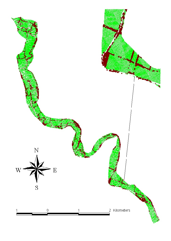
Solutions to these problems proposed by the Environment Agency (1997) include that the errors associated with the transformation from WGS84 to OSGB36 can be eliminated by displaying the z values as WGS84 and only transforming the x and y co-ordinates which would improve the z accuracy greatly. This would, however, invalidate comparisons with standard topographic data sets, such as the one being used in this study, which are usually in the OSGB36 co-ordinate system. It is also suggested that the use of at least two GPS ground stations would allow cross referencing of positional data during post-processing of the aircraft position and help to eliminate spurious offsets and act as a quality control measure. Finally, to remove vegetation, the data was gridded and a simple variance filter applied to identify data points that measured the height of the trees, hedgerows and other floodplain features such as houses instead of the underlying topography (Environment Agency, 1997). The statistical variance around each grid cell was calculated using a 3 x 3 filter producing a new surface containing grid cells above a specified variance threshold of 180,000 mm, selected using trial and error. This was 'grown' slightly by producing a 5m buffer around each grid cell to ensure all hedgerow and woodland segments are linked resulting in a mask that can be overlain onto the gridded LIDAR data to remove any cell values thought to be due to floodplain features rather than actual topography. Whilst this method will inevitably lead to some loss of resolution and may fail to remove a small percentage of the vegetation-affected values, it would seem a reasonable initial attempt to deal with this complex issue. Ultimately, however, a scanning LIDAR that returns, as a minimum, first and last return information is required for many environmental applications including floodplain hydraulic modelling. The mask resulting from this procedure is shown in Figure 1.
Figure 1 - Mask delineating elevation values containing spurious topographic floodplain features, typically vegetation (shown in brown) from land surface elevation values (shown in green).
The LIDAR elevation data used in this study related to a section of the River Stour floodplain upstream of Blandford Forum in Dorset. This was obtained on the 5th December 1996 as part of the test program conducted by the Environment Agency and was used to provide a partial topographic parameterisation of a reach approximately 12 km in length and 500 m wide between the gauging stations at Hamoon and Blandford Forum. The original data consisted of a 5 x 7 km block of approximately 4 million individual elevation values, recorded as x, y and z measurements in the OSGB36 co-ordinate system. Bounding of the domain to represent the floodplain only reduced the number of measurements to 300 000 and the gridding and removal of points thought to incorporate vegetation height measurements further reduced the final topographic data set, prior to integration with the model, to 261 634 elevation values. This represents a point density of approximately 64 600 topographic measurements per km2 or a horizontal resolution of ~ 4 m and compares favourably with the 3 contour lines and 20 spot heights falling within the floodplain area in the standard topographic data set. For areas of the 12 km reach outside the range of the LIDAR flight path the standard topographic parameterisation previously described was used to complete the coverage.
The model selected for application to this reach was the TELEMAC-2D finite element scheme as it is an example of a complex hydraulic model where the model resolution attainable in reach scale studies (and required for process investigations) has previously been in excess of the available topographic data (Bates et al., 1996, Bates et al., 1992). TELEMAC-2D is a hydrodynamic simulation model developed by the Départment Laboratoire National d'Hydraulique (LNH) at Electricité de France, Direction Études et Recherches (EDF-DER). The model solves the St. Venant or Shallow Water Equations, which are the depth-averaged version of the full three-dimensional Navier Stokes equations. Extensive numerical (Hervouet and Janin (1994), Hervouet and Van Haren (1996)) and process validation studies (Cooper, 1996) have shown that TELEMAC-2D is a well-specified code suited to a number of hydraulic modelling scenarios. The model has also been tested against other two-dimensional finite element codes and has been found to offer superior capabilities in the prediction of bulk flow and in the simulation of a realistic range of inundation extents, (Bates et al., 1997, Bates et al., 1995).
A high resolution finite element mesh consisting of 11 265 linear triangles and 6049 computational nodes was developed for the River Stour reach between the flow gauging stations at Hamoon (upstream) and Blandford Forum (downstream). The mesh discretisation was designed to maximise the density of nodes on the floodplain and consequently used only five nodes to represent the channel cross section. This is appropriate for a numerical model used as a flood simulator as we are only concerned with flows above bankful discharge. Hence, we merely wish to replicate channel volume such that the onset of flooding is correctly simulated rather than model detailed in-channel flow patterns. The average side length of each element was therefore 26.8 m and overall the mesh represents the current computational maximum for dynamic flood simulations at this scale performed on a high powered workstation.
The standard and LIDAR-derived DEM data sets were interpolated onto the above mesh using a linear inverse distance weighting of the 4 data points closest to each node to produce an average interpolated value for the nodal elevation. This method is appropriate for the 10 x 10 m DEM at this mesh resolution, however the LIDAR data produces approximately 40 points to each node resulting in a high degree of data redundancy. This was, however, unavoidable as we wished to obtain a consistent processing method for both data sets which therefore needed to be appropriate for the lowest resolution data. Channel topography was assigned from 25 surveyed cross sections made available by the UK Environment Agency and values linearly interpolated between these points. The cross sections were however concentrated primarily in the upper and lower portions of the reach thus the channel long profile in the middle of the reach was specified by linear interpolation over much longer length scales than in the upper and lower reach areas.
An identical TELEMAC-2D set up was used for each simulation. This employed a fractional step method (Marchuk, 1975) where advection terms are solved initially, separate from propagation, diffusion and source terms which are solved together in a second step. For the advection step several schemes may be chosen with the Method of Characteristics chosen here for the momentum equation. To ensure mass conservation and oscillation-free solutions with unrefined meshes the Streamline Upwind Petrov Galerkin (SUPG) method (Brookes and Hughes, 1982) was applied for the advection of the water depth, h, in the continuity equation. According to this technique, standard Galerkin weighting functions are modified by adding a streamline upwind perturbation, a method which overcomes problems of artificially diffuse solutions produced by ordinary upwinding methods. The second step (propagation) made use of an implicit time discretisation and solved the resulting system with a conjugate gradient type method.
Boundary conditions for each model consisted of an imposed flow rate at the upstream inflow and an imposed water surface elevation at the downstream outflow. This combination gives a well posed problem according to the theory of Characteristics providing that there is no recirculation at the downstream outflow. Initial conditions for each simulation were assumed to be steady state flow at bankful discharge calculated using identical friction parameters to those employed in the dynamic simulation. Steady state conditions were calculated by the model for each site commencing with a uniform water depth at each node. Non-dynamic boundary conditions representing bankful discharge were then imposed and a simulation made which proceeded until any waves created by the start-up procedure had passed out of the domain. In the case of the standard parameterisation this procedure led to water contained in the channel only and floodplain areas fully dry. The complexity of the LIDAR topography meant that at this scale some ponding of water on the floodplain, covering 8% of the total valley floor area, remained at the start of the simulation and could not be removed.
A 1 in 4 year recurrence interval flood which took place over 62 hours on and around 20 December 1993 was simulated. This was discretised into 55 800 time steps each with a duration of 4 s. Preliminary simulations were undertaken to determine appropriate friction parameters which discriminated between channel and floodplain areas. This approach was chosen as the only items of model-independent observed flow data were bankful discharge at the up- and downstream gauging stations and the timing of the downstream discharge peak. While water level and discharge data existed at the downstream gauge, the former were used as a model boundary condition and the latter was subject to additional uncertainties due to the rating equation. As a consequence only the timing of peak discharge was accurately known and independent of the model. Calibration was therefore achieved by manipulating friction parameters solely to correctly replicate the onset of flooding and minimise the phase error between predicted and observed peak discharge. This has the advantage of providing a relatively robust test of the model as all other aspects of the hydrograph (volume, magnitude of peak, timing and speed of rise, timing and attenuation of recession) were allowed to vary freely. Final values for the friction parameters used were 0.017 for the channel and 0.035 for the floodplain.
Simulations were compared in terms of the differences between the two topographic parameterisations and the respective patterns of flow throughout the flood event. These two criteria are linked as hydraulic flood routing is particularly sensitive to changes in the topographic parameterisation and feedback (positive or negative) may well occur where changes in topography have a knock-on effect on the flow patterns predicted further downstream in the model. The topographic parameterisations were compared using a difference surface between the standard and LIDAR-derived topographic parameterisations (Figure 2). Hydraulic flow patterns were analysed using time sequences of inundation extent.
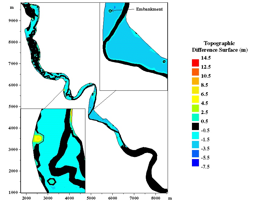
Figure 2 - A plot of the differences between the standard and LIDAR topographic surface parameterisations where positive values indicate a higher LIDAR elevation measurement.
Figure 2 shows values for the difference between the two topographies calculated by subtracting the elevation value for each node in the standard parameterisation from the value for the same node in the LIDAR parameterisation. This results in a surface where a negative value represents a point with a lower LIDAR elevation value than the standard elevation value. The differences range from a few areas where the LIDAR elevation value is up to 14.4 m higher than the standard topography to the majority of areas where it is up to 7.5 m lower. Differences that are greater than ± 0.5 m cover approximately 50% of the floodplain domain and the resulting surface is, on average, 1 to 3 m lower than the standard topographic surface. The majority of this area of lower topography occurs in the middle of the reach although there are also areas of lower topography of the same magnitude present in the upper reach albeit to a lesser extent. These differences are broadly consistent with the quoted error for each data set given above.
There is a small area of difference between the two surfaces of approximately 1.25 m which is located where a railway embankment crosses the floodplain perpendicular to the channel (upper right insert, Figure 2). The embankment is not present at all in the standard topographic surface, hence the difference between the two parameterisations, and this emphasises that the denser coverage of the LIDAR data offers the potential to detect floodplain topographic features that the smoother standard parameterisation may miss. Despite having identified this feature, the LIDAR data is only partially successful in mapping its whole length. This occurs as a result of the removal of a part of the embankment elevation data by the variance method for vegetation extraction previously described, as the embankment values display a variance above the threshold value for most of the length of the bank. In effect, the processing method confuses 'real' topography with vegetation and removes points it designates (incorrectly) as spurious. Other areas where the LIDAR parameterisation has elevation values that are significantly lower than the standard topographic floodplain are observed along the edges of the floodplain domain and tend to be confined to the upper reach. These represent regions where the standard parameterisation includes the elevation of side slopes bordering the floodplain. It seems likely that smoothing of the real topography in the standard perturbation leads to higher elevation values being assigned to areas that are actually part of the valley floor.
Areas where the LIDAR data provides a higher parameter value than the standard topographic parameterisation tend to be isolated points randomly located throughout the reach. These points are probably a consequence of inadequacies in the vegetation removal method where a tree or part of an actual hedgerow may have been incorrectly identified as ground. This results in a locally unrealistic representation of the floodplain surface which may subsequently impact upon the prediction of flood inundation extent. However, these areas are relatively few in number, being less than 5% of the total floodplain area. Figure 2 also shows the extent of the area of common topography which results, as discussed previously, from the LIDAR data for the reach being incomplete and extends for approximately the final 4 km of the model domain. This also has the additional benefit of acting as a control surface for an analysis of the feedback effects of the new topographic parameterisation on the floodplain hydraulics and flow routing.
A dry floodplain could not be achieved under steady state conditions in the model prior to the flood simulation using the LIDAR data. This may result from either the differences in elevation values already noted between the new LIDAR topographic surface and the standard topographic parameterisation or from the use of the original channel cross-section data or a combination of both. Despite being collected by ground survey, and hence probably of high accuracy, the cross-sections used to parameterise the channel were only available for the upper and lower reaches of the model domain with the mid-reach channel section being an interpolatant of this data. In attempting to gain a steady state condition in the model, it was noted that the areas most affected by ponding were adjacent to this middle section. Closer examination revealed the presence of some distinct jumps in the elevation value between channel and top of bank, causing steep gradients to be present in the model's representation of the channel cross-section. This may result in a localised change in the channel volume and thus affect the point at which bankful discharge occurs at this point in the model domain. However, as noted previously, this area of data deficiency with regards to channel cross-sections also coincides with a much lower floodplain topography as measured by the LIDAR sensor which will also cause water to pond. It is therefore probable that many of the problems experienced in attempting to gain a dry floodplain prior to modelling the flood event are as a result of the interaction of the interpolated channel cross-section with the lower floodplain topography. This causes the water to overtop the bank as it enters the middle of the reach but limits drainage back into the river channel. In order to facilitate an accurate comparison between the two topographic parameterisations, the flood simulation was started with this partially wet floodplain (approximately 8% of the floodplain inundated to a depth greater than 0.1 m) as removal of water prior to the simulation would have necessitated either adjusting bank node elevations and/or the channel flow volume, which would invalidate the study.
During the simulation, similar inundation patterns were observed in the upper portion of the reach and the slight differences that were obtained can be seen to reflect the areas of difference between the two topographic parameterisations. In the middle of the reach, where the topographic parameterisations show the maximum difference, an increase in water depth on the already inundated floodplain occurs in the LIDAR parameterised model. This happens at the same timestep in both simulations as shown in Figure 3. Subsequently, the water drains back into the channel but, due primarily to the presence of depressions on the floodplain, ponding is observed in several areas of the LIDAR parameterisation and the water recedes more slowly than in the standard model. At the end of the simulation, the inundated area covers a slightly smaller percentage of the floodplain than at the start of the simulation in both model parameterisations but proportionally, the flood in the LIDAR parameterisation has not decreased as much.
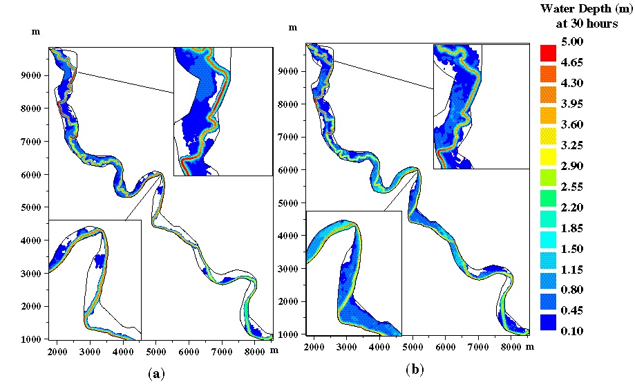
Figure 3 - Comparison of predicted water depth in the model at maximum inundation extent using standard topography (a) versus using LIDAR topography (b).
The model's sensitivity to topographic parmeterisation is demonstrated by the difference in flood inundation extent observed throughout the simulation on the common topographic parameterisation at the end of the reach. The use of the standard topography in both simulations acts as a control to enable upstream feedback effects to be identified. Figure 4 shows very little flood inundation in this area in the simulation which uses the standard topographic parameterisation whilst the substantial inundation in the middle reach in the LIDAR parameterised simulation is seen to cause additional inundation to occur further downstream on the area of standard topography. Such knock on effects are consistent with previous theoretical studies (Bates and Anderson, 1996) and is demonstrated here for the first time using actual topographic data. This indicates the care which needs to be taken in the construction of high dimension, high resolution hydraulic schemes.
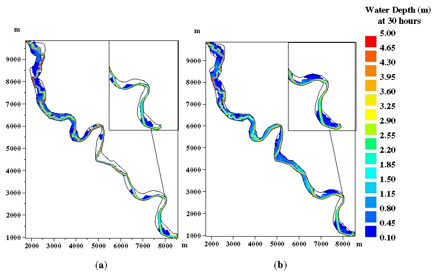
Figure 4 - Comparison of predicted water depth in the model at maximum inundation extent illustrating the model's sensitivity to topographic change using standard topography (a) versus using LIDAR topography (b).
The model's sensitivity to topographic change can be considered both in terms of the change in the bulk characteristics of the floodwave (such as the outflow hydrograph and percentage inundation extent) and the local hydraulics of the flow (flow velocities and depths at the nodes and patterns of inundation). Whilst the time taken for the floodwave to pass through the reach is the same for both simulations (shown by peak inundation extent occurring at the same timestep in Figure 3), the physical processes within the simulation are changed and this directly affects the local hydraulics throughout the model. These physical process changes may potentially be further reinforced by a feedback mechanism which may be very difficult to isolate. Thus the inundation observed only in the LIDAR parameterised simulation on the area of topography common to both simulations occurs as a result of changed flow processes on the differing topographies further upstream.
This paper has presented results of a comparison between standard methods of parameterising topographic data in reach scale two-dimensional finite element hydraulic models and novel high-resolution LIDAR data. It was demonstrated that flood hydraulics are directly affected by even quite small changes in topography and the model sensitivity was more complex than might have been expected. In particular, topographic change in the upper or middle reaches resulted in increased inundation further down the reach in areas where the local topography was identical.
The primary advantage of the LIDAR data was its accurate digital nature which was less subject to the horizontal errors inherent in using data sets derived from contour lines. Other advantages include its rapid collection and the future possibility of repeat flights over floodplains which can be subject to sudden topographic change in the event of a flood, thus opening the way for a study into the temporal change of the floodplain.
Two problems in the use of such data for the hydraulic modelling of floodplain flow are, however, outlined in this paper. Primarily, the dense coverage of the LIDAR data set leads to a large degree of data redundancy with around 250 000 measurements being available from which to assign elevation values to 6049 model nodal points. Secondly, this redundancy is further compounded by the use of an unsophisticated interpolation method for the integration into the model of the data, whereby only a small number of topographic points (four per model node) are actually used to assign the elevation value to a given nodal point. We therefore require better methods of integrating the local topography from a relatively large sample of points into a single composite value. Further research is also required to assess the quantity of data required to achieve particular simulation objectives with a given level of accuracy. This will require the specification of mesh resolution and data quality and quantity required for a given application such that the simulation remains computationally efficient. Research is also required into the efficient representation of the floodplain surface through the application of advanced interpolation methods which fully utilise the topographic information available.
The availability of these data sets now facilitates a move to a wider usage of two-dimensional hydraulic models which were previously constrained by a lack of topographic data for parameterisation. A full comparison of the use of the new high-resolution data sets against traditional data sets in these models will require high quality inundation extent data which is as yet unavailable. However, this paper has demonstrated the immediate utility in using a two dimensional approach to represent the spatial complexity of flow processes throughout the floodplain and thus it is likely that such models will be fully utilised in the future as data commensurate with (or in excess of) the typical model resolution becomes available. But in order to fully utilise any topographic data set, better representation of the complex surface is required at the level of the individual application of the model and this will become increasingly important as data sets continue to increase in resolution and coverage. This will be achieved through a process beginning with an improvement in the current interpolation procedures used by the model pre-processor for integrating the topographic data into the model but will ultimately require regenerating the mesh adaptively based on the topography rather than the present independent mesh design.
The authors would like to thank the UK Environment Agency and the UK Ordnance Survey for the provision of data used in this study. Kate Marks was funded under NERC Studentship GT4/96/23/F.
Anderson, M.G. and Bates, P.D. (1994). 'Initial testing of a two dimensional finite element model for floodplain inundation'. Proceedings of the Royal Society of London, Series A, 444, 149-159.
Bates, P.D. and Anderson, M.G. (1993). A two-dimensional finite-element model for river flow inundation. Proceedings of the Royal Society of London - Series A 440, 481-491.
Bates, P.D. and Anderson, M.G. (1996). A preliminary investigation into the impact of initial conditions on flood inundation predictions using a time/space distributed sensitivity analysis. Catena, 26, 115-134.
Bates, P.D., Anderson, M.G., Baird, L., Walling, D.E. and Simm, D. (1992). 'Modelling floodplain flow with a two dimensional finite element scheme'. Earth Surface Processes and Landforms, 17, 575-588.
Bates, P.D., Anderson, M.G. and Hervouet, J.-M. (1995). 'An initial comparison of two 2-dimensional finite element codes for river flood simulation'. Proc. Instn. Civ. Engrs., Wat., Marit. and Energy, 112, 238-248.
Bates, P.D., Anderson, M.G., Price, D., Hardy, R.J. and Smith. C.N. (1996). 'Analysis and development of hydraulic models for floodplain flows'. In Anderson, M.G., Walling, D.E. and Bates, P.D. (Eds.), Floodplain Processes, John Wiley and Sons, Chichester, 215-254.
Bates, P.D., Stewart, M.D., Siggers, G.B., Smith, C.N., Hervouet, J.-M., and Sellin, R.H.J. (1998). Internal and external validation of a two-dimensional finite element code for river flood simulations. Proceedings of the Institution of Civil Engineers - Water, Maritime and Energy (in press).
Biggin, D.S. and Blyth, K. (1996). A Comparison of ERS-1 Satellite Radar and Aerial Photography for River Flood Mapping. Journal of the Chartered Institute of Water and Environmental Management 10, 59-64.
Brackett, R.A., Arvidson, R.E., Izenberg, N.R., and Saatchi, S.S. (1995). Use of Polarmetric and Interferometric Radar Data for Flood Routing Models: First Results for the Missouri River. Session 36 - Planetary Geology: Radar Remote Sensing of Flood Plains, Mountain Belts, and Volcanos. Annual Meeting of the Geological Society of America, 5-9th November 1995, New Orleans, USA.
Brookes, A.N. and Hughes, T.J.R., (1982). 'Streamline Upwind/Petrov Galerkin formulations for convection dominated flows with particular emphasis on the incompressible Navier-Stokes equations'. Computer Methods in Applied Mechanics and Engineering, 32, 199-259.
Cooper, A.J. (1993). TELEMAC-2D Version 3.0 - Validation Document. (Report EDF-LNH HE-43/96/006/A). 74 pages.
Environment Agency - National Centre for Environmental Data and Surveillance (1997). Evaluation of the LIDAR technique to produce elevation data for use within the Agency.
Feldhaus , R., Höttges, J., Brockhaus, T. and Rouvé, G. (1992). 'Finite element simulation of flow and pollution transport applied to a part of the River Rhine'. In: Falconer, R.A,. Shiono, K. and Matthews, R.G.S (Eds.), Hydraulic and environmental Modelling; Estuarine and River Waters, Ashgate Publishing, Aldershot, 323-344.
Flood, M. and Gutelius, B. (1997). Commercial Implications of Topographic Terrain Mapping Using Scanning Airborne Laser Radar. Photogrammetric Engineering and Remote Sensing 63 (4, April), 327-366.
Gee, D.M., Anderson, M.G. and Baird, L. (1990). 'Large scale floodplain modelling'. Earth Surface Processes and Landforms, 15, 512-523.
Hervouet, J.-M. and Janin, J.-M. (1994). Finite Element Algorithms for Modelling Flood Propagation. In: Molinaro, P. and Natale, L. (Eds.), Modelling of Flood Propagation Over Initially Dry Areas. American Society of Civil Engineers, New York, 102-113.
Hervouet, J-M. and Van Haren, L. (1996). Recent Advances in Numerical Methods for Fluid flow. In Anderson, M.G., Walling, D.E. and Bates, P.D (Eds.), Floodplain Processes, John Wiley and Sons, Chichester, 183-214.
Krabill, W.B., Collins, J.G., Link, L.E., Swift, R.N and Butler, M.L., (1984). 'Airborne laser topographic mapping results'. Photogrammetric Engineering and Remote Sensing, 50, 685-694.
Lin, C.S. (1997). Waveform sampling lidar applications in complex terrain. International Journal of Remote Sensing 18 (10), 2087-2104.
Marchuk, G.I. (1975). 'Methods of numerical mathematics', Springer-Verlag, New York, 316pp.
Ritchie, J.C. (1996). Remote sensing applications to hydrology: airborne laser altimeters. Hydrological Sciences Journal 41 (4, August), 625-636.
Ritchie, J.C., Menenti, M., and Weltz, M.A. (1996). Measurements of land surface features using an airborne laser altimeter: the HAPEX-Sahel experiment. International Journal of Remote Sensing 17 (18), 3705-3724.
Ritchie, J.C., Jackson, T.J., Garbrecht, J.D., Grissinger, E.H., Murphey, J.B., Everitt, J.H., Escobar, D.E., Davis, M.R., and Weltz, M.A. (1993). Studies using an airborne laser altimeter to measure landscape properties. Hydrological Sciences Journal 38 (5, October), 403-416.
Samuels, P.G. (1990). Cross section location in one-dimensional models. In White, W.R. (Ed.) International Conference on River Flood Hydraulics. John Wiley, Chichester, 1990, 339 - 350.
Samuels, P.G. (1985). 'Modelling of river and flood plain flow using the finite element method'. Hydraulics Research Ltd., Technical Report SR61, Wallingford.