Mark Gahegan and Geoff West
School of Computing, Curtin University of Technology, PO Box U 1987, Perth 6845, Australia.
Email: mark@cs.curtin.edu.au, geoff@cs.curtin.edu.au
This paper presents an overview of the functioning, control, reporting and analysis capabilities of two of the popular Artificial Intelligence techniques that are used in geocomputation as tools for classification; namely decision trees and artificial neural networks. The strengths and weaknesses of both techniques are described with respect to their operational foundation primarily, as opposed to simply contrasting results obtained. The mathematical foundation behind the two methods is not described in detail as others have fully explored these aspects.
These techniques each use a different approach to locate some minimum error or entropy solution to the standard classification problem, via strictly defined mechanisms. However, their application to geocomputational problems is often conducted in a rather haphazard fashion, which in turn can lead to unreliable results. This paper attempts to explain the classification problems encountered in geocomputation as they relate to the above techniques. Many of the datasets used are characterised by a high degree of inherent complexity, often including several layers of data, gathered according to a variety of statistical scales. Such datasets offer significant classification challenges that defy a casual approach using existing off-the-shelf tools or packages, but instead require careful consideration based on sound operational (and sometimes theoretical) knowledge of the tools to be used.
The use of decision trees and artificial neural networks for data classification in geography and remote sensing has seen a steady rise in popularity. Bishof et al. (1992), Kamata and Kawaguchi (1993) and Civco (1993) describe neural network classifiers whilst Lees and Ritman (1991), Eklund et al. (1994) and Freidl and Brodley (1997) describe classification approaches based around decision trees. Initially, the focus of attention was on comparing classifier performance with established methods (e.g. Benediktsson, et al., 1990; Hepner et al., 1990; Paola and Schowengerdt, 1995; Fitzgerald and Lees, 1994). More recent efforts have concentrated on methodologies and customisation that improve performance or reliability; a sign that the technology has reached at least some level of acceptance. For example, Benediktsson, et al., (1993) and German et al. (1997) describe performance improvements and Kanellopoulos and Wilkinson (1997) and Gahegan et al. (1998) address methodological issues from the specific viewpoint of geographic datasets.
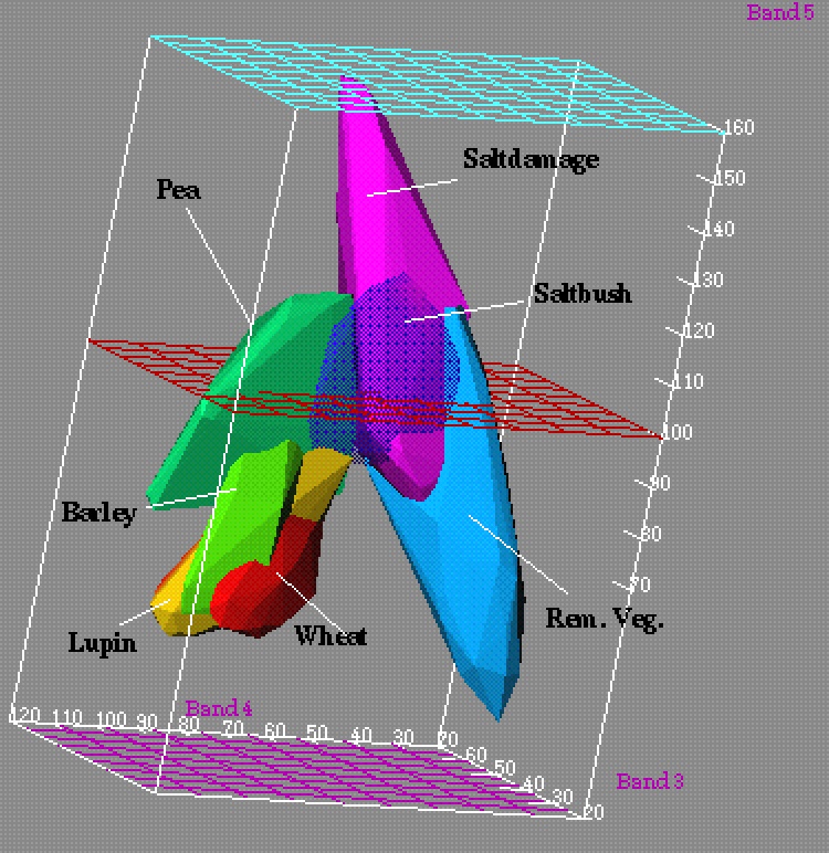
The kinds of classification problems that arise in geography or the wider earth sciences are often characterised by their complexity, both in terms of the classes and the datasets used. For example, classes may be difficult to define, may vary with location and over time, and their properties may overlap in attribute space. Figure 1 shows an example from remote sensing in which classes overlap and are difficult to separate.
Datasets increasingly contain many descriptive variables (layers) and often contain a mix of statistical types; for example remotely sensed reflectance values (quantitative data) supplemented with nominal data such as soil type or geology and ordinal data such as slope or aspect. Data 'saturation' seems set to increase with the adoption of sensing devices of greater sophistication, resulting in a higher spatial resolution and many more channels. The complexity of the tasks to which these data are applied is also increasing; for example the classification of deep geological structure from 300 channel airborne electro-magnetics data.
In this paper the classification problem is discussed concentrating on supervised classification. This is followed by brief descriptions of neural networks and decision trees. The descriptions only cover the basic principles along with how they are configured for the supervised classification task. The main part of the paper then deals with a number of assumptions and goals that have not been discussed at length in the literature, namely the formulation of attribute space, generalisation capabilities and obtaining good or 'optimal' classifiers. Finally, some comparisons are made between the two methods from a geocomputational perspective.
Figure 1. A three dimensional attribute space comprised of three channels of Landsat TM data. The coloured volumes represent convex hulls formed around training data for identified landcover classes from an agricultural mapping exercise. Some of the classes overlap, indicating problems with separability. One class (Saltbush) has been rendered with a degree of transparency so that its intersection with other classes can be studied.
Classification is a common task that achieves two distinct purposes. Firstly it is a data reduction technique, used to reduce a complex dataset into a form where it can be manipulated straightforwardly; for example, by using the map algebra provided by most analytical GIS. Secondly, it is a transformation technique, mapping data to a thematic model of space, where the themes or classes are defined by the user to represent entities of semantic importance to a specific domain (Gahegan, 1996). The overall effect is thus one of generalisation, essential to human reasoning. A good classification should both impose structure and reveal the structure already present within the data (Anderberg, 1973).
The mapping of inputs (the attribute values) to outputs (the desired class labels) would ideally be conducted analytically. Where the problem becomes too complex for an analytic solution (such as is described above) we must resort to the use of heuristic approaches, exemplified by such AI techniques as inductive machine learning. This paper compares the approach to the classification of geographic datasets taken by neural networks and decision trees by explaining how the attribute space is constructed and partitioned. Specifically, differences in the generalising abilities of the two approaches are described.
Classifiers can be divided into two groups, supervised and unsupervised. Supervised techniques have a training phase during which samples of data representing the chosen classes are used to establish a model for the classification process. Unsupervised techniques do not require training or any pre-conceived notion of a class, being based purely on grouping or clustering the data, usually formulated on the Euclidean metric. The discussion in this paper is restricted to supervised classifiers only. In other words, given a number of examples of mappings from input attributes to output classes, the task of supervised learning is to generalise over the mappings to produce one general mapping from input attributes to output classes.
A supervised classification procedure consists of a number of steps. Note that, irrespective of the actual classifier being applied, the procedure is largely identical. So, a similar type of approach is required for decision trees, neural networks and the more traditional Maximum Likelihood Classification (MLC). The following procedure is based loosely on that given by Richards (1986), but modified to provide a validation step after training but prior to final classification.
Throughout the following discussion, it should be borne in mind that the choice and use of a specific classifier largely affects step 3 and has only minor impact on the other steps. However, the biggest limiting factors are likely to hinge around steps 1 and 2; specifically, the differentiability of classes is largely a product of how carefully the classes are chosen in the first place and how well the attributes both characterise them and support their discernment. The user may not have much choice over such matters in practice.
Classification involves the partitioning of attribute space, the various parts of which can then be identified with the desired output class. Neural networks and decision trees partition the attribute space via a series of discrimination functions - within neural networks these are referred to as hyperplanes and in decision trees as decision rules or cuts. In both techniques it is a summation of these functions that define the partitions. A description of each technique follows.
Artificial neural networks are often referred to colloquially as 'universal function approximators', because of their ability to model mathematical relationships and complex mappings in a heuristic manner. There are a number of ways of interpreting the internal behaviour of a neural network (e.g. Carpenter, 1989; Kohonen, 1989). In a multi-layer perceptron such as shown in Figure 2, which has 5 attributes, 6 hidden nodes and 3 classes, one interpretation is based on mapping input attribute values to output classes, and applies to the typical backpropagation feedforward neural network (e.g. Rumelhart and McClelland, 1986; Pao, 1989).
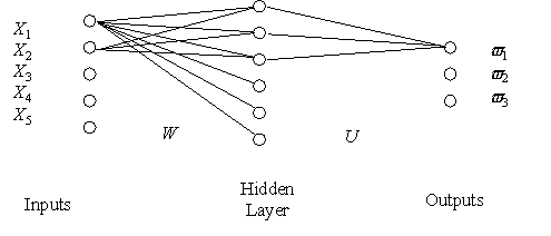
Figure 2. A typical neural network architecture. For clarity, the diagram shows only some of the connections, whereas each node in the hidden layer is connected to all input and output nodes.
The attribute values applied to the network are evaluated with each hyperplane parameterisation to determine the algebraic distance from each hyperplane. The algebraic distance for a plane in 3-D space is given by: algebraic_distance = ax + by + cz + d, where (a, b, c, d) are the coefficients of the plane in (x, y, z) space as shown in Figure 3. The hyperplane parameters (a, b, c, d) are values in the weight vector W that maps the input values to nodes in the hidden layer.
The equation for algebraic distance is derived from the equation of a plane in which a point on the plane is defined by: ax + by + cz + d = 0.
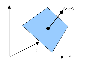
Figure 3. Illustration of algebraic distance.
For a plane, the algebraic distance is equivalent to the Euclidean distance from a point to the plane defined by the perpendicular from the point to the plane. Note that for other hypersurfaces e.g. hyperconics, this is not the case. A measure of which class a sample belongs to can be determined using the algebraic distances. One method is to determine on which side of each hyperplane the sample falls which is indicated by whether the algebraic distance is +ve or -ve. This approach is used in linear classifiers. A second method is to sum the algebraic distances and use these to indicate the class. This is the scheme used in typical neural networks.
For the two attribute case, Figure 4 shows a possible set of hyperplanes that can give good performance. The resulting algebraic distances at the hidden nodes are combined together via a non-linear function and the matrix U to map to the required class output. So, the hyperplanes fragment the space into many part-classified regions which can then be summed on output and assigned to the appropriate class. So it is the weighted combination of discriminant functions that provide the class descriptions. Hence, the many distinct regions shown in Figure 4 can be combined where they represent the same class, so only two classes (squares and diamonds) are produced.
Ideally, for an example of class v 1, the attributes Xj for j = 1, ..., 5 should map to {1, 0, 0} for v i where i = 1, ..., 3. Any deviation from this ideal represents classification 'error', which the network attempts to minimise over the entire training data set.
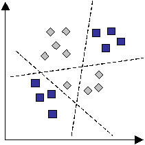
Figure 4. Hyperplanes in a neural network.
The weights between the three layers (matrices W and U in Figure 2) are determined in some minimum error sense to achieve the best mappings for the set of training samples. An error function could be defined as:
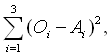
where Oi for i = 1, ..., 3 are the outputs of the network for one input which should be the same as Ii for i = 1, ..., 3 for the chosen class e.g. I = {1, 0, 0}. For example, it may be the case that I = {0.9, 0.2, 0.3} in which case the error is used to modify the values of W and U to reduce the error. Given an error criterion such as described above, a global minimum is searched for such that the error produced over all samples and classes is minimised. Whether the global minimum is found depends on the initial conditions for the search (the weights W and U are usually set randomly) and the complexity of the error space (presence of many local minima).
The use of algebraic distance in neural networks means that generally they produce a continuous output, which can be regarded as a 'soft' classification where each training example has a finite likelihood of belonging to each class, much the same as the posterior probabilities given by the MLC. The output must be mapped to discrete class labels, usually by selecting the dominant output value.
Note that in this standard configuration, the neural network is unable to distinguish between cases where the dominant value is correct and where it is not. As a consequence, the network is penalised for any residual values on all but the desired output node (the values 0.2 and 0.3 in the above case). Given that classes are often not entirely separable anyway, such a penalty may be unreasonable and cause oscillation in the hyperplane positioning as the network tries to increase the value on the appropriate output node.
Decision trees decompose the attribute space into P disjoint subsets, Kr, r = 1, ... P, using decision rules (cuts) that are usually orthogonal to the attribute axes (axis parallel). Thus a decision rule can be described by a simple expression of the form ai ³ Ti, or ai < Ti, where Ti is some threshold, making their operation easy to comprehend by the user. Figure 4 shows part of a decision tree along with the rules that occur at each node. Given labelled attribute data, decision trees choose the most appropriate attributes with which to partition the feature space to give the best classification performance. Figure 5 shows a 'normal' decision tree (C4.5: Quinlan, 1993) that only uses attribute values.
In Figure 4, each node in the tree makes a binary decision based on one (or more) attribute values. Attributes can occur anywhere in the tree and the leaves define final decisions as to the chosen classes.
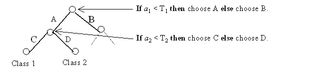
Figure 5. The operation of a simple decision tree.
The classification of a region in a decision tree is determined by the path described from the root of the tree to a leaf. Hence, each rule progressively refines the classification in a hierarchical manner. The tree reflects the complexity of the classification problem; many rules are used for classes where separation is problematic, and few where it is easy, so the tree only becomes complex (deep) where it is necessary. Likewise, only attributes that appear to aid the classification problem are considered when rules are defined; other attributes are simply ignored. The usual way for the tree to be built is as follows. Starting at the root, all attributes are tested to see which one is the best for splitting the data into two disjoint sets. The best attribute is the one that partitions the data such that the minimum number of samples are misclassified (see Section 8.2). After this stage, the tree consists of two branches and one root node. For each branch the process is repeated to build the tree, partitioning the samples to further improve the partitioning of the data.
The fact that the cuts are axis parallel as shown in Figure 6, and are conducted in a sequence has some implications for generalisation and optimisation (see later). Some decision trees, such as OC1 (Murthy et al, 1994) can use a non-orthogonal splitting rule (oblique), which is based on perturbing the best orthogonal cut to see if the performance of the rule can be improved.
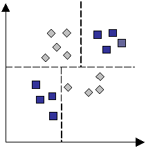
Figure 6. Decision tree partitioning of attribute space showing the axis-parallel planes. Compare with the planes of Figure 4.
The attribute space required by a decision tree or neural network (or an MLC) is simply a space of dimensionality n, where n is the number of attributes being used. So, each attribute supplies a single dimension. Both techniques are what might be referred to as 'distribution free' in that they make no assumption as to the shape or form of the distribution of training data within the attribute space. In fact, statistical assumptions are reduced to a minimum, the only assumption retained relating to the attribute space is that Euclidean distance within this space has meaning, with smaller distances implying a greater degree of similarity and larger distances a greater degree of difference.
The training samples are considered to be independent of each other. When using neural networks it is common practice to scale (normalise) the attributes, so that the range of values within each domain is consistent, usually such that 0 £ a £ 1. This is necessary because attributes are used in combination, so must be numerically comparable. (Also, without this, precision problems may arise within the computer due to the rounding of values.) No such problem occurs with decision trees because each splitting rule is formulated on a single attribute in isolation. The only comparison required is that of performance between the various decisions that could be made for each attribute type.
When the attribute space is initially constructed, no allowance is made for dependence that might naturally be present (such as height being correlated with temperature or aspect being correlated with rainfall). The weighting of evidence, so that the relative contribution of each attribute type as a means of identifying a class, is learned by a neural network during the training phase. Decision trees implicitly weight evidence by ordering rules according to the improvement that associated split brings to overall performance. Attributes with poor qualifying power are either ignored or are used only deep within the tree.
It is often claimed that, unlike parametrically based classifiers, neural network and decision tree classifiers can function without difficulty on data of any statistical type, so the individual attribute dimensions can represent a mixture of nominal, ordinal and quantitative (interval and ratio) data types. However, to achieve this the nominally valued attributes must be enumerated so that they may be mapped to an axis, giving rise to some ordering issues as illustrated in Figure 7. Specifically, the separation complexity (the number of rules/planes needed to produce the required classification accuracy) is dependent on how this nominal data is 'ordered' when enumerated. Consider the case where several nominal values {A, B, C, D, E, F} encode some condition such as soil type, three of which {A, B, C} are indicators of a particular landcover class, shown as the squares in Figure 7. Depending on the ordering of these values, the number of decision boundaries required might vary between 1 and 6. Of course, an entirely different ordering may be appropriate when trying to identify each of the other target landcover classes!
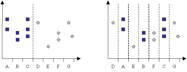
Figure 7. Two different orderings for the nominal dataset {A,B,C,D,E,F,G} in a two-class problem.
When using neural networks, this assignment problem further complicates the task of determining the correct number of hyperplanes required. With decision trees, the problem is more subtle in its manifestation; if the soil types are separated then the individual improvement they are each able to offer, if used as the basis of a split, will be reduced, and may even become insignificant. One conclusion is that if nominal data shows a consistent clustering for all target classes then it should be merged or ordered accordingly, to simplify the classification task.
Any attributes relating to space or time are usually included in the overall attribute space in the same straightforward manner, so they have no special significance as far as the classifier is concerned. The utility of positional data can often be improved by separating out the x, y (and possibly z and t) components and encoding them separately, since this simplifies the task of clustering the data in geographic space. Alternatively, a spatial addressing technique that has a natural clustering property, such as Morton or Hilbert coding (e.g. Worboys, 1995) can be used to transform separate x, y (z, t) attributes into a single variable on which spatial clustering can still be performed efficiently. As with the nominal data example given above, the complexity of the separation problem depends on the effectiveness of the mapping of data to the axes.
The positioning of the boundaries to achieve the best generalisation to the validation data, without over- or under-fitting remains problematic. The issue that needs to be addressed may be understood by reference to least and most generalisation. Figure 8(a-b) shows the two cases for two attributes and two classes. Most generalisation is a discriminator as it makes a decision based on which side of each partition the sample falls. For example: If the value of x is less than T then it belongs to class w1 else it belongs to class w2. In other words the attributes are unbounded. Least generalisation is a descriptor with the attribute values localising the samples in some parallelepiped in attribute space and the spaces between the parallelepipeds ignored. For example: If the value of x is between T1 and T2 then it belongs to class w1 else it is unknown. In other words the attributes are bounded. Most generalisation is appropriate if it can be confidently assumed that the training data are representative of the situation such that all future data values do fall into one of the classes. However least generalisation is better for situations in which the training data only partially represent the real world. For example, other classes may occur that are not in the training set and least generalisation allows an unknown class to be implicitly used without having training samples. Figure 8(b) gives an example of least generalisation introducing the concept of an unknown or background class into areas of the attribute space where training examples are absent.
Least generalisation is of interest because the attributes for a sample must have the correct values to be classified, whereas the attribute values are irrelevant for most generalisation so long as the sample falls on the correct side of the partitions. Using either form of generalisation, it is still entirely possible that large regions in the attribute space contain no supporting examples from the training data, but data falling in them are still assigned to a specific class. As an example, consider a sample to be classified that falls some distance from identified classes, such as the star shown in Figure 8(a-c).
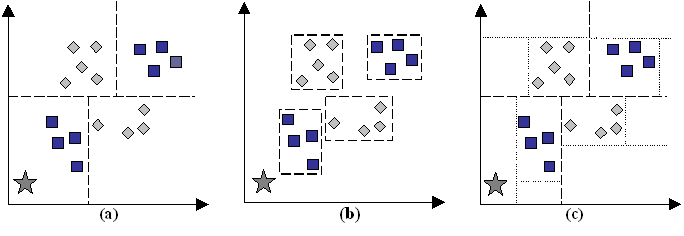
Figure 8. Most generalisation (a), least generalisation (b), and hybrid generalisation (c). The star represents an unknown sample to be classified. It is included in the 'square' class in (a) because it falls within the class decision boundary, but is excluded from (b) and (c) because it is unlike any square previously encountered.
Neural networks position hyperplanes freely within a continuous attribute space, with the ultimate position being determined by the search for a (hopefully) global error minimisation, as described above in Section 4. Usually, they employ most generalisation, since the hyperplanes will be positioned to maximise class separation. Overtraining occurs when the network starts to focus on minimising error due not to significant trends within the data, but on the individual nuances of the particular set of attribute values found in the training set, i.e. tending towards least generalisation. This can occur when too many hyperplanes are introduced in the hope of reducing error. Overtraining is difficult to detect except by periodically evaluating the performance of the classifier on the validation set.
By contrast decision trees can be set up to use either approach. Given an ordered, finite set of training examples {v1, v2, ... vm}, a decision boundary (vI) can be placed anywhere between vi and vi+1. Decision boundaries close-to or coincident with vi will cause least generalisation of the class which the vI split helps to define.
Least generalisation in decision trees usually employs the smallest bounding hyperectangles to define the boundaries, carrying with it the same problems as overtraining in neural networks. As Figure 8 shows, there may be situations where this type of least generalisation may still involve an act of faith! Compare this with the approach to least generalisation shown in Figure 1 where each convex hull has been constructed in 3D attribute space to encompass all samples for that class. This can be supported directly if oblique decision rules are allowed, otherwise it must be approximated by employing (usually a great many) extra rules.
A trade off between least and most generalisation may offer a good balance between the characteristics of the two cases. A variety of alternative statistical techniques could be employed here, as described by Devijver and Kittler (1982). Extreme value theory (Castillo, 1988; Matthews, 1996) is one technique that has not been explored and may be able to model the distributions within each parallelepiped to decide on the positions of the partition boundaries. One possibility is shown in Figure 8(c) which is generated by using most generalisation to build an initial decision tree after which the attribute values for each leaf are examined and bounds introduced based on the training data. The leaves of the tree are then modified with further decisions to reflect these bounds without re-building the tree from scratch (McCabe et al., 1998).
Clearly, it is important to match the generalising abilities of the classifier to the patterns observed within the data, although there is no straightforward mechanism by which this can be achieved, hence the need for experimentation and validation before the final classification stage.
The following sections deal with some of the practical issues that arise when using these classifiers. They are based on our own experiences and those of our colleagues. We have deliberately chosen to not include specific results by way of a comparison, because the number of issues described and the complexity involved in setting up the classifiers makes a direct contrast rather meaningless. Nevertheless, we have accumulated a good many sets of results that back up the discussion below, and will make these available to other researchers on request.
Both techniques can easily accommodate the idea of a sub-class (a class composed of two or more disjoint regions within the attribute space). When using decision trees, the existence of such is no longer a cause for concern for the user since the decision tree simply uses as many rules as are required to provide the necessary partitioning. For neural networks the situation is a little more complex, since the isolation of sub-classes requires the availability of additional hyperplanes with which to describe the separate regions and also the ability to position hyperplanes around the problematic areas in attribute space.
Binary classifications, for example forest and not forest from landcover data, are likely to produce large numbers of subclasses, i.e. for each landcover type in the 'catch all' class not forest. The choice of generalisation method (Section 7) can then become very important since accuracy depends on how well a single class can be delineated. There is some evidence to suggest that decision trees may perform better than neural networks for this type of problem (Evans et al., 1998). This could be due to two reasons: (i) decision trees allow the type of generalisation to be selected by the user, and (ii) it may be difficult to select the correct number of hyperplanes when using neural networks, especially if the training data gives no hint as to the number of classes in the 'catch all' set.
Within a neural network, there are a number of crucial architectural decisions that can have a dramatic effect on performance; solutions to many of these for the standard multi-layer perceptron feedforward network using back propagation are described by Gahegan and German (1996). However, the selection of the number of hyperplanes (ie. the number of hidden layer nodes) is critical to success. Too few hyperplanes will not allow full separation of all classes, too many hyperplanes and the network is likely to over-train (see Section 7), resulting in poor generalisation capabilities. The problem facing the user is that it is not possible to know, prior to use, exactly how many are required, hence the necessity to exhaustively test various network configurations to find one that appears to perform well on validation. Clearly, this is both a computational burden and source of annoyance for the user.
More recent developments in the neural network literature attempt to address this weakness, either by proposing alternative, more adaptive architectures (Grossberg, 1991) or by trying to identify, for each pairwise class separation sub-problem, exactly how many nodes are needed and how they can be brought into operation as and when required (German et al., 1998).
Decision trees too suffer from a similar problem, albeit with less problematic consequences. The criterion used to determine when a class is adequately described has been the subject of much research. The thresholds used for each decision are chosen using minimum entropy or minimum error measures. The minimum entropy method was originally proposed by Hunt (1966) and used by Quinlan (1993) in C4.5. It is based on using the minimum number of bits to describe each decision at a node in the tree based on the frequency of each class at the node. Alternatively, some minimum error function based on statistics or algebraic distance can be used, although this is not popular in decision trees. With minimum entropy, a stopping criterion is needed which is based on the amount of information gained by a rule (the gain ratio). This threshold is set by the user, again by experimentation. Experiments on the gain ratio show it can help to build robust and smaller trees (Quinlan, 1993). The advantage that decision trees enjoy is that refinement is simply a matter of continuing the classification process, rather than starting again with a different number of hyperplanes.
Neural networks attempt to examine all dimensions at once in their quest for an 'optimal' solution and have sophisticated search routines which examine error trends in an attempt to find the global minimum (point of least overall error), as described in Section 4. These routines can be made sensitive to the gradient and direction of change (Benediktsson et al., 1993). However, it is still not possible to guarantee that the global minimum has been found (unless the surface is exhaustively searched which requires an analytic method).
By contrast, decision trees move toward a solution incrementally, making an independent decision in a single data dimension at each iteration. The order in which the decision rules are generated determines how the error surface is searched and is dictated by the data alone. Hence, decision trees do not have a concept of a global minimum (although some systems can plan the next n moves in advance).
So, neither technique can promise to find the optimal solution, even under ideal conditions (where the 'correct' number of hyperplanes or the stopping criterion is known). Therefore, classifier performance can only be evaluated reliably with respect to statistically independent validation data. Trying to predict performance based on the ability to classify the data used for training is likely to result in an inflated view of accuracy, since no account of overtraining (Section 7) can be taken.
Since we aim to use these techniques on complex datasets, where the number of input layers and / or output classes is high, we must examine how the computational complexity and performance (in terms of computing time) are affected as the attribute and class space grows.
Decision trees must determine the best attribute and threshold on which to split at each node. Attribute data are sorted into order and all possible thresholds are tested for performance gain. The overall complexity is highly dependent on the data although experience with real problems shows the sorting to be the major factor-- although the time to build a tree is in of the order of seconds for even large datasets. However, the complexity of the problem rises only linearly with the number of dimensions within the attribute space, due to the independence of rules as described above in the previous section.
For neural networks, the issue of complexity is more complex. The search mechanism is effectively global, searching all attributes and classes simultaneously (Section 8.1). So we might expect a squared relationship between attributes and computing demands as the dimensionality of the search problem is increased. However, this is not the case. Each additional dimension attracts one extra input node, and hence q extra weight connections to the hidden layer (where q is the number of hidden layer nodes). This complicates the task of training in terms of the W matrix (Section 4). However, if the number of hyperplanes required does not increase, then again the performance increase is approximately linear. It is when new hidden layer nodes are added that complexity rises alarmingly, since this affects both W and U. But even then, the use of sophisticated searching procedures (Section 8.3) reduces the impact of the change, so that complexity falls somewhere between a linear and a squared relationship with the number of attributes.
In practice, we have found that, for decision trees, scalability causes no problems. For neural networks, we have had to invest a good deal of effort into architectural issues. This is due largely not to computational complexity, but to 'saturation' of the hidden layer nodes; a problem that occurs when there are a large number of input nodes to connect to. The more weights there are, the harder it is to ensure that only useful evidence is passed on. Training too can become very time consuming, particularly if the network is initialised randomly to begin with. The neural network package DONNET (http://www.cs.curtin.edu.au/~gisweb/donnet) strives to overcome these problems by setting the weights based on linear discriminants and using scaled conjugate gradient descent.
This paper has addressed issues in the choice and design of two of the most popular machine learning techniques currently available. Issues addressed include generalisation and a number of operational issues such as architecture, searching for the solution and complexity. Many of these issues are not taken into account when classifiers are used. The adoption of these tools over existing methods boils down to this single question "Which is best, learning a distribution imperfectly or using a predefined distribution that may be unsuitable?" Obviously, the answer to this question depends on the data under consideration. In our experience performance gains can be substantial on complex problems and also not worth the effort on simple ones.
Decision trees and neural networks are not a panacea for all the ills of existing parametric classifiers, neither does their use guarantee an increase in accuracy. Whilst they can, to a limited extent, overcome some of the difficulties of more established methods, they introduce problems of their own, namely: computational performance, generalisation behaviour and configuration. However it is important to note they have and can be used as black box classifiers by users albeit with the danger of not knowing their characteristics. Certainly, these tools require a good deal more of the user, particularly in the selection of operational parameters. This points to the need for experimentation followed by validation on independent data. If the complexity of the classification task is completely unknown, then decision trees may present the best alternative, since they are simpler to configure.
For complex (deep) attribute spaces, the global searching employed by neural networks seems to facilitate better classification performance, although this increase in accuracy is usually paid for through a good deal of experimentation to find a suitable network configuration. For example, DONNET (Section 8.4) performs about 10% better than C4.5 on the Kioloa Pathfinder Dataset. (DONNET achieves an accuracy on validation of around 70-75%). Both methods outperform maximum likelihood methods considerably (these typically produce about 40% classification). For comparison, Figures 9, 10 and 11 show typical examples.
The difficulty of deciding which is the best classifier and what parameters are appropriate have lead to the declaration of four 'open problems' by Dietterich (1997) of which three are relevant here. These are (1) using ensembles of classifiers to improve performance, (2) scaling up supervised learning algorithms, and (3) learning complex stochastic models (such as causal probabilistic networks). Ensembles of classifiers can consist of a number of different decision tree and neural network classifiers whose outputs are combined in some way to give better classification eg. by majority voting. Scaling up is concerned with the problem of learning over training sets of millions of samples, and stochastic models advance from the use of simple statistical models such as unimodal Gaussian distributions. These issues show that there is still a good deal of ground to cover in our collective efforts to provide more robust classification tools for the geosciences.
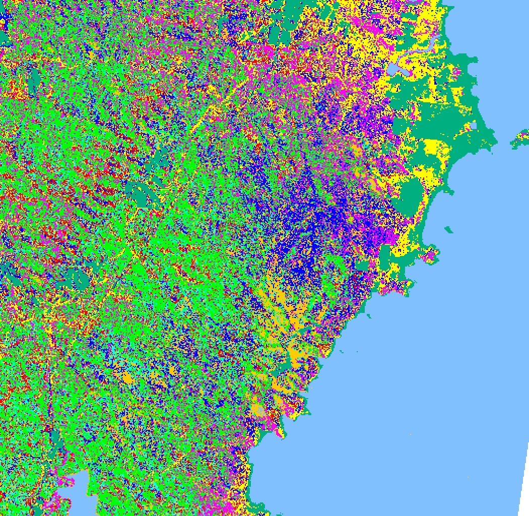
Figure 9. Maximum likelihood classification gives poor performance on this complex dataset-- note the severe fragmentation of most landcover classes. The multivariate Gaussian distribution used by the classifier provides an inadequate model. The data is taken from the Kioloa area of the New South Wales coast, Australia. Key: yellow-- Dry sclerophyll, dark blue-- E.botryoides, red-- lowerslope wet, bright green-- wet E.maculata, purple, dry E.maculata, mid blue-- rainforest ecotone, orange-- rainforest, jade green-- cleared land (pasture), light blue-- water.
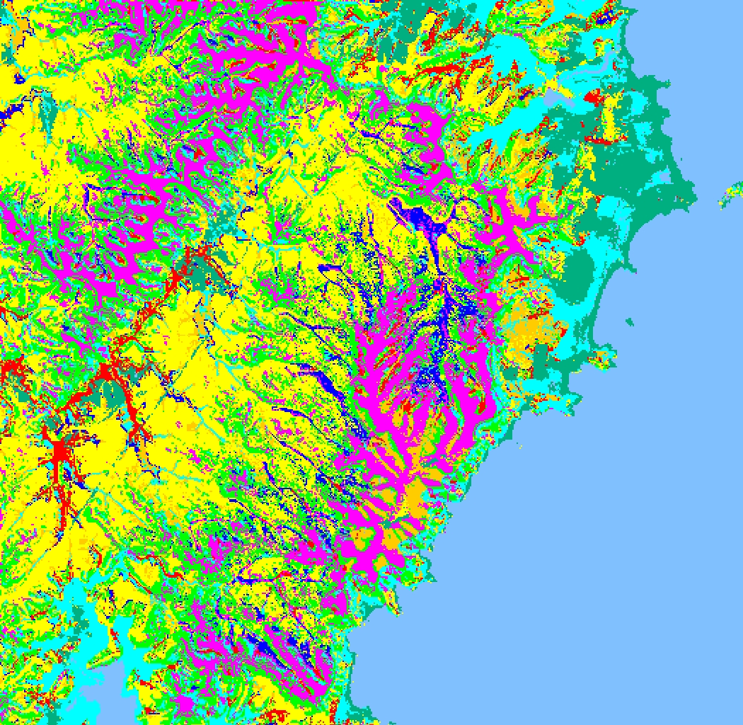
Figure 10. Classification of the Kioloa Dataset using a decision tree (C4.5) gives a considerable improvement, although some detail is missing, particularly with respect to poorly separable classes which mainly inhabit the steep valleys running NW to SE in the scene. The ability of the decision tree to manage sub-classes is a significant factor in performance improvement over Figure 9.
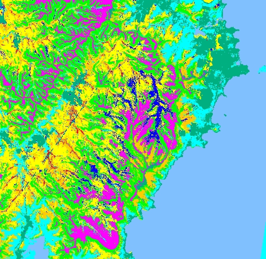
Figure 11. Classification of the Kioloa Dataset using a neural network (DONNET). The performance on the steep valley regions is improved over those in Figure 10-- more of the floristic structure is evident. On this dataset, a neural network achieved the best results, due in part to its more flexible approach to hyperplane positioning.
Anderberg, M. R. (1973). Cluster Analysis for Applications, Academic Press, Boston, USA.
Benediktsson, J. A., Swain, P. H. and Ersoy, O. K. (1990). Neural network approaches versus statistical methods in classification of multisource remote sensing data. IEEE transactions on Geoscience and Remote Sensing, Vol. 28, No. 4, pp. 540-551.
Benediktsson, J. A., Swain, P. H. and Ersoy, O. K. (1993). Conjugate gradient neural networks in classification of multisource and very high dimensional remote sensing data. International Journal of Remote Sensing, Vol. 14, No. 15, pp. 2883-2903.
Briscoe, G. and Caelli, T. (1996). A Compendium of Machine Learning (volume 1: Symbolic Machine Learning). Ablex Publishing Corp., Norwood, New Jersey, USA.
Carpenter, G. A. (1989). Neural network models for pattern recognition. Neural Networks, Vol. 2, pp 243-257.
Castillo, E., (1988). Extreme Value Theory in Engineering, Academic Press, Boston, USA..
Civco, D. L. (1993). Artificial neural networks for landcover classification and mapping. International Journal of Geographical Information Systems, Vol. 7, No. 2, pp. 173-186.
Devijver, P. A. and Kittler, J. (1982). Pattern Recognition: A Statistical Approach. Prentice-Hall International Inc, London.
Dietterich, T. G. (1997). Machine learning directions, AAAI AI Magazine, pp. 97-136, winter.
Eklund, P. W., Kirkby, S. D. and Salim, A. (1994). A framework for incremental knowledge update from additional data coverages. Proc. 7th Australasian Remote Sensing Conference, Melbourne, Australia, Remote Sensing and Photogrammetry Association of Australia, pp. 367-374.
Evans, F. H., Kiiveri, H. T., West, G. and Gahegan, M. (1998). Mapping salinity using decision trees and conditional probabilistic networks, Proc. Second IEEE International Conference on Intelligent Processing Systems, Gold Coast, Queensland, Australia.
Fitzgerald, R. W. and Lees, B. G. (1994). Assessing the classification accuracy of multisource remote sensing data. Remote Sensing of the Environment, Vol. 47, pp. 362-368.
Freidl, M. A. and Brodley, C. E. (1997). Decision tree classification of land cover from remotely sensed data. International Journal of Remote Sensing, Vol. 61, No, 4, pp. 399-409.
Gahegan, M. N. (1996). Specifying the transformations within and between geographic data models. Transactions in GIS, Vol. 1, No. 2, pp. 137-152.
Gahegan, M., German, G. and West, G. (1998). Some solutions to neural network configuration problems for the classification of complex geographic datasets. To appear in Geographical Systems.
German, G. and Gahegan, M. (1996). Neural network architectures for the classification of temporal image sequences. Computers and Geosciences, Vol. 22, No. 9, pp. 969-979.
German, G., Gahegan, M. and West, G. (1997). Predictive assessment of neural network classifiers for applications in GIS. Second International Conference on GeoComputation, Otago, New Zealand, pp. 41-50.
German, G., Gahegan, M. and West, G. (1998). Improving the Learning Abilities of a Neural Network-based Geocomputational Classifier. Proc. ISPRS Symposium II, Cambridge, UK. ISPRS Publications.
Grossberg, S. (1991). Neural Pattern Discrimination, In: (Carpenter, G. A. and Grossberg, S., eds.) Pattern Recognition by Self-Organising Neural Networks, MIT Press, Cambridge, MA, USA, pp. 111-156.
Hepner, G. F., Logan, T., Ritter, N. and Bryant, N. (1990) Artificial neural network classification using a minimal training set: comparison to conventional supervised classification. Photogrammetric Engineering and Remote Sensing, Vol. 56, No. 5, pp. 469-473.
Hunt, E. B., Marin, J. and Stone, P. J. (1966). Experiments in Induction. Academic Press, New York, USA.
Kamata, S. and Kawaguchi, E. (1993). A neural network classifier for multi-temporal Landsat images using spatial and spectral information. Proc. IEEE 1993 International Joint Conference on Neural Networks, Vol. 3, pp. 2199-2202.
Kanellopoulos, I. and Wilkinson, G. (1997). Strategies and best practice for neural network image classification. International Journal of Remote Sensing, Vol. 61, No, 4, pp. ???
Kohonen, T. (1989) Self organisation and associative memory (3rd edition). Springer-Verlag, Berlin, Germany.
Lees, B. G. and Ritman, K. (1991). Decision tree and rule induction approach to integration of remotely sensed and GIS data in mapping vegetation in disturbed or hilly environments. Environmental Management, Vol. 15, pp. 823-831.
Murthy, S., Kasif, S. and Salzberg, S. (1994). A system for induction of oblique decision trees, Journal of Artificial Intelligence Research, vol. 2, pp. 1-32.
McCabe, A. (1998). Hybrid most and least generalisation with C4.5, Technical Report 3/98, School of Computing, Curtin University of Technology, Perth, Western Australia.
Matthews, R. (1996). Far out forecasting, New Scientist, No. 2051, 12th October, pp. 37-40.
Pao, Y. H. (1989). Adaptive pattern recognition and neural networks. Addison-Wesley, Reading, Mass. USA.
Paola, J. D. and Schowengerdt, R. A. (1995). A detailed comparison of backpropagation neural networks and maximum likelihood classifiers for urban landuse classification. IEEE transactions on Geoscience and Remote Sensing, Vol. 33, No. 4, pp. 981-996.
Quinlan, R. (1993). C4.5: Programs for Machine Learning, Morgan Kaufmann, San Mateo, California, USA.
Richards, J. A. (1986). Remote Sensing Digital Image Analysis. Springer-Verlag, Berlin, Germany.
Rumelhart, D. E. and McClelland, J. (1986). Parallel Distributed Processing. MIT Press, Cambridge, MA, USA.
Worboys, M. F. (1995). GIS: A Computing Perspective. Taylor & Francis, London.