|
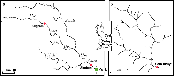
| Figure 1: Location map for the (a) River Ouse and (b) Upper River Wye catchments |
Linda See1, Robert J. Abrahart2 & Stan Openshaw1
1Centre for Computational Geography
School of Geography, University of Leeds, UK.
Email: {l.see}{stan}@geog.leeds.ac.uk
2Department of Geography, University College Cork, Ireland.
Email: bob@ashville.demon.co.uk
This paper presents four different methodologies for integrating conventional and AI-based methods to provide a hybridised solution to the problem of generating continuous river flow and flood forecasting estimates. Individual models ranging from neural networks to statistical predictors were developed on a standalone basis using historical time series data for gauging stations on the River Ouse in North Yorkshire and the Upper River Wye in Central Wales. A simple linguistic fuzzy logic model for Skelton, and TOPMODEL predictions for the Upper Wye, were also incorporated as additional model inputs. Each of these individual models were then integrated using four different approaches: an averaging procedure, a Bayesian approach, and two fuzzy logic models, the first based on just current and past river flow conditions, and the second on a fuzzification of the crisp Bayesian approach. Model performance was assessed via global statistics and more specific flood related evaluation measures. The addition of fuzzy logic to the crisp Bayesian model yielded overall results that were superior to both the individual model estimates and the other integrated approaches.
Artificial intelligence (AI) techniques, and the integration of these methods to provide a soft computing (SC) solution, can now be used to model complex problems in both the physical and social sciences. These intelligent computational methods, which include artificial neural networks, fuzzy logic and genetic algorithms (Openshaw & Openshaw, 1997), offer real advantages over conventional modelling, including the ability to handle large amounts of dynamic, non-linear or noisy data, and such tools can be especially useful when the underlying relationships are not fully understood. Other associated benefits would include improved performance, faster model development and calculation times, and improved opportunities to provide estimates of prediction confidence through comprehensive bootstrapping operations. When used alone, each of these techniques can be extremely effective, but when utilised together, the individual strengths of each approach can be exploited in a synergistic manner for the construction of powerful hybrid intelligent systems. It is also possible to go one step further and couple these new methods with conventional mathematical and statistical tools in an extended hybridisation. The potential to produce a more flexible, more adaptive and less assumption dependent solution is therefore large. Wherever possible, in appropriate circumstances, these systems should also utilise the knowledge of experts and attempt to incorporate the imprecision and uncertainty associated with various aspects of the modelling problem.
Despite having a vast range of potential benefits, AI and SC still remain somewhat unexplored areas within environmental science. For instance, in hydrological research, the majority of effort has to date been concentrated on the straightforward application of backpropagation neural networks to 'one-step-ahead' river flow prediction tasks; e.g. Karunanithi et al. (1994) have demonstrated how a neural network can be used to estimate flows at an ungauged site for assessing stream change effects on fish habitats, and Hsu et al. (1995) have shown that a neural network outperforms both an ARMAX model and the conceptual lumped Sacramento Model for the prediction of streamflow on a medium sized basin in Mississippi. Other applications have demonstrated that neural networks can be used successfully to model synthetic data generated from existing conventional models (e.g. French et al., 1992; Smith & Eli, 1995; Minns & Hall, 1996). Neural networks could also be used as plug-in replacement components, or as a direct substitute for conventional models, since their calculation times, once trained, are considerably faster. The UK Ministry of Agriculture Forestry and Fisheries (MAFF) has also shown interest in the potential of neural networks, specifically in the context of enhancing the performance and reliability of conventional flood forecasting systems, and as a tool for aiding in the design of future computer-based systems. To investigate these questions a MAFF-funded 18 month feasibility study was recently undertaken at the School of Geography, University of Leeds, working in collaboration with the UK Environment Agency (EA). Results from this work indicated that neural networks developed for the River Ouse catchment outperformed both statistical predictors and the River Flow Forecasting System (RFFS), a conceptualmodel used in this region by the EA, when modelling a series of historical storm events (Openshaw et al., 1998).
All of these examples demonstrate the potential power of using neural network-based approaches for continuous river flow prediction. But the development of a fully operational AI-based rainfall-runoff model, or a set of standalone tools that could be used alongside an existing forecasting and warning system to produce additional predictions, is still some way off. This gap in the toolbase reflects the early stages of AI-based research in hydrology. A great deal more empirical experimentation into the application of these technologies to hydrological modelling will be required before these approaches are established as accepted methodologies, especially among those hydrologists who would appear to have moved away from inductive black-box models, in favour of more physically-based ones. Moreover, there is little or no research being done on the integration of different methods, encompassing both AI-based and conventional modelling approaches, to produce a hybrid formulation. The potential benefits that might be obtained through combining the many different, but complementary approaches, into a single integrated system still requires assessment.
This paper presents a hydrological application that was developed in parallel with the MAFF-funded neural network feasibility project, which combines fuzzy logic and neural networks, with mathematical and statistical-based modelling, to form an integrated river flow forecasting system. Historical times series data for gauging stations at the base of the River Ouse catchment (Yorkshire) and the Upper River Wye basin (Wales), both in the United Kingdom, were used to demonstrate the methods. Neural networks, ARMA models and naive predictions were first developed for both sites. Additional river flow predictions were also obtained from a fuzzy logic model developed for the Ouse, and from TOPMODEL for the Upper Wye. Four different approaches were then used to link the individual models into a single forecasting system:
The predictions produced by these methodologies were assessed using (a) global performance statistics and (b) more specific flood related evaluation measures. The combined results were also compared with those of the individual models developed on the same dataset.
The two areas that were chosen to investigate the different prediction abilities of these integrated approaches were (a) the River Ouse in Yorkshire and (b) the Upper River Wye in Central Wales (Figure 1). The Ouse catchment, which covers an area of 3,286 km2, encompasses an assorted mixture of urban and rural land uses. Gauging stations are distributed throughout the catchment along each of its three main tributaries: the Nidd, the Swale and the Ure. Four years worth of hourly data (1989-92) from the gauging station at Skelton were used. This station has a downstream location, situated far from the headwaters of the catchment, and the river at this point has a relatively stable regime. The use of a six hour forecasting horizon was therefore considered reasonable.
The Upper Wye catchment, on the other hand, is much smaller in size. It comprises an upland research basin that has been used on several previous occasions for various hydrological modelling purposes (e.g. Bathurst (1986); Quinn & Beven (1993)). The basin covers an area of some 10.55 km2, elevations range from 350-700 m above sea level, and average annual rainfall is in the order of 2500 mm. Ground cover comprises grass or moorland and soil profiles are thin, most of the area being peat, overlying a podzol or similar type of soil (Knapp, 1970; Newson, 1976). Hourly data were available from the gauging station at Cefn Brwyn for the three year period 1984-6. In contrast to Skelton, this small catchment has a quick response time, and the modelling operation was therefore implemented on a 'one-step ahead' prediction basis.
The individual and hybrid methodologies were therefore tested on data from two different stations, that are situated in two contrasting catchments, which is reflected in the decision to use different forecasting horizons.

|
| Figure 1: Location map for the (a) River Ouse and (b) Upper River Wye catchments |
Previous work on river flow prediction for the Ouse at Skelton has focused on the development of a hybrid neural network (HNN), an ARMA model and naive predictions using data for the period 1989 to 1992. The HNN consists of five individual feedforward networks that were trained on five different hydrograph event types, where an event is a section of a hydrograph such as low flow, high peak, etc. The event types were determined by partitioning historical level data with a self organizing map (SOM) classifier (Kohenen, 1985). The five neural networks were then reintegrated into a single hybrid model via a simple fuzzy logic model that determines which weighted combination of network predictions to use for a given set of river level conditions. The full particulars of this work, and on each item therein, are provided in See & Openshaw (1998). In addition to these three methods, a simple linguistic fuzzy model (SLFM) has also been developed to provide another set of individual model inputs. Five input variables were employed to build the SLFM predictor and each variable was partitioned into three fuzzy sets. In order to avoid the 'rule explosion' problem that can occur when the number of input variables and fuzzy sets increases, the number of variables and fuzzy set partitions was kept to a minimum . The five model inputs were:
This choice of input variables represents the minimum number that are needed to provide adequate information regarding direction and magnitude of the predicted river levels. The use of upstream data from each of the tributaries is analogous to a simple routing model or transfer function. It is unfortunate that conventional predictions of this nature were not available for either comparison or direct incorporation. The output variable, which was the change in river level in six hours time, was partitioned into nine fuzzy sets which was considered a sufficient number to provide for adequate patching of the solution space. Rather than classify the data via a SOM and recombine the individual models, as in the HNN formulation, a genetic algorithm was used to train the fuzzy model on an equal proportion of the different occurrences of the five original hydrograph types found within the training dataset. Based on this decision, only 30% of the training records were in fact used in the model optimisation process, which diminished the common bias that exists towards low level events. The SLFM output for the entire training dataset produced an RMSE value of 0.109 m; the RMSE value was actually higher for the subset of the data used in the optimisation process (0.120 m) since there was an equal representation of event types. The SLFM output for the validation dataset produced an RMSE value of 0.110 m.
Overall the SLFM results were worse than the ARMA predictor but considerably better than the naive predictions. Full details are provided in Table 5 (see results section). The SLFM model seems to suffer from the same problem as a global neural network solution, in that it must be able to characterise many hydrograph responses within a single model, whilst at the same time having to use just a small number of fuzzy sets. The overall model performance is however surprisingly good given these particular and exacting constraints. The other important consideration, from a flood forecasting perspective, is how well the SLFM predictor might capture certain features of the hydrograph. For example, if the fuzzy model were to outperform the other models on any one particular aspect of the hydrograph, then its predictions could still be useful in a multi-model solution. So, with this in mind, it is evident that the true potential of the fuzzy logic model will emerge when examining the proposed hybrid solutions.
Unfortunately, no outputs were available for the RFFS, since this conceptual model is designed to operate in real-time; indeed, even the generation of a single historical six hour ahead prediction was a time consuming exercise, and generating the complete historical data record (which is somewhere in the region of 35,000 observations) would have been a near impossible task given the limited time constraints of the MAFF-funded project and this associated research. However, it should be emphasised that all types of model prediction can be integrated into the multi-model solutions that are presented here, including those from the RFFS if these had been to hand. In order to test the potential of this method using RFFS predictions, it would require linking the multi-model solutions to the RFFS in real-time. This is possible - at least in a theoretical sense - via the construction of a standalone multi-model program that has a direct numerical link to the existing RFFS software. The development and testing of such a system remains an area for further investigation.
A lot of previous research has been undertaken on the Upper Wye catchment and it therefore made good sense to build upon this work via the incorporation of a recognised mathematical model into the model integration process. Previous modelling experiments have been undertaken using TOPMODEL and are reported in Beven et al. (1984) and Quinn & Beven (1993). TOPMODEL is a physically-based process model that was developed in the late '70s and its last reported implementation to the Upper Wye catchment in 1993 was restricted to the nine snow-free months (April-December). With help from an experienced TOPMODEL user we therefore sought to reproduce this work and in so doing created a set of useful outputs for our model integration operation. TOPMODEL was calibrated on 1985 data and additional predictions were computed for 1984 and 1986, this work being performed in a more or less identical manner to the 1993 application (Lamb, personnel communication). Since TOPMODEL predictions were only available for 9 months, the integrated models used the other individual model predictions for the remaining 3 months. Three individual neural network solutions were included: the first network was created using standard backpropagation training procedures (NN1); the other two networks were the result of automated pruning exercises that were used to create smaller and better performing networks (NN2 and NN3). NN2 was created using magnitude based pruning while NN3 was developed with a skeletonization pruning algorithm. It should be noted that the network solutions were created using a full twelve month set of 1985 training data and an optimal solution was selected from a visual inspection of changes in the error associated with the other two periods. Further particulars on the construction and performance of these various network solutions is provided in Abrahart et al.(1998). In addition, an ARMA model was developed on a full set of 1985 data, and validated with the other two years. Naive predictions, which use the value at the last time step as the current prediction, were also calculated for the entire time period.
At this point it must be stressed that there is a fundamental difference between the mechanisms that created the TOPMODEL output and the other predictions. TOPMODEL output was based on a continuous run with no updating of the river flow values (Beven, personnel communication; Lamb, personnel communication). The model is run in an iterative manner. Each prediction is therefore susceptible to the influence of accumulated error propagation. The other models were producing 'one-step-ahead' predictions based on constant update which therefore excluded the knock on effect of cumulative erroneous predictions. We would therefore expect a higher level of performance, in most cases, from the 'one-step-ahead' predictors. This is not to denigrate the performance of TOPMODEL, which, if we were comparing like with like, would in all likelihood produce the best results over longer forecasting horizons. For example, in comparison to a neural network, superior results have been observed at t+12, t+24 and t+48 hours (Abrahart, 1998).
In a real-time forecasting situation, each of these individual models would be running as an independent standalone system, with the multi-model program running in the background, and integrating the various predictions as and when these individual estimates became available. However, in order to develop the multi-model solutions off-line, a database was created containing each of the individual model predictions for all training and validation data periods. For Skelton, the first 60% of the four year record was used to train the models while the remaining 40% was used as a validation dataset; for the Upper Wye, 1985 records were used as the training dataset, while the other two years were used for validation. Four different approaches were then taken to integrate the predictions. In the first case, a simple average of the four individual model results was calculated and this value was then used as the prediction. This averaging method is based on the hypothesis that better predictions might be obtained if the patterns of residuals exhibited by the different models do in fact cancel each other out when averaged. The success of this method relies on the models having contrasting patterns of residuals (Dougherty, personal communication).
In the second multi-model solution, the Bayesian approach of Dougherty (1997) was used, which employs the simple rule that the model which performed the best at the last time step is the one chosen to make the next prediction. In contrast to the fuzzy Bayesian approach described below, this is a crisp implementation or crisp Bayesian model (CBM). Tables 1 and 2 list the percentage of the time that each model produced the best performance on both the training and the validation datasets. For Skelton, the individual HNN model performed the best at the last time step more often than any of the other methods. However, the second best performer was the SLFM predictor, which was slightly better than the ARMA model despite having a poorer overall performance in terms of RMS error. Thus, in a multi-model context, the SLFM is useful. The naive predictions were also better than the others almost 20% of the time, demonstrating that even the simplest method of prediction can be a useful one at times, particularly if the main concern is not just about making flood forecasts.
| Individual Model | Training | Validation |
|---|---|---|
| HNN | 36.2 | 33.6 |
| ARMA | 21.1 | 22.2 |
| SLFM | 23.5 | 26.4 |
| Naive | 19.2 | 17.8 |
For the Upper Wye (Table 2), the ARMA model dominates, followed by the naive predictions, and then each of the neural network solutions. TOPMODEL gives the best performance for the smallest amount of time which is not at all surprising since, as mentioned earlier, this model does not include real-time updating.
| Individual Model | 1984 | 1985 | 1986 |
|---|---|---|---|
| TOPMODEL | 1.2 | 3.0 | 2.7 |
| NN1 | 4.4 | 9.7 | 8.1 |
| NN2 | 6.8 | 6.6 | 6.9 |
| NN3 | 8.1 | 5.9 | 5.3 |
| ARMA | 60.3 | 55.3 | 60.1 |
| Naive | 19.2 | 19.5 | 16.9 |
For the remaining two approaches, fuzzy logic-based multi-model solutions were developed. Each of these used a set of simple IF-THEN rules to determine which model should be run based on current conditions and past model performance. Since all rules fire in parallel, more than one model may be recommended, but to varying degrees, with the final outcome being a weighted average of the individual model recommendations. A genetic algorithm was used to optimise each fuzzy model. In the first method, referred to as the fuzzy master model (FMM), the current water level and the change in water level over the last six hours were used as inputs to determine which of the models to recommend. In the second approach, the crisp Bayesian method was fuzzified, resulting in a more generalised multi-modelling approach. Rather than just choosing the best performing model at each time step, the fuzzy-Bayesian model (FBM) used the current water level, and the prediction error at the last time step between the observed level and each of the model predictions, to recommend which models to use at the current time step. The fuzzy FBM predictor has a distinct advantage over the crisp CBM approach in that it can recommend more than one 'good' performing model at a given time instead of being forced to pick a single best solution. This approach also allows for the selection of those models which are best suited to a given set of flow or level conditions, potentially producing a more sensitive forecasting system. The final input membership functions for both fuzzy models are provided in Figures 2 and 3 for Skelton and Figures 4 and 5 for the Upper Wye.
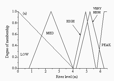 | 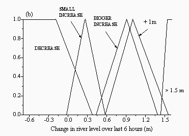 |
| Figure 2: Membership functions for the inputs: (a) current level and (b) change in level for the FMM for Skelton | |
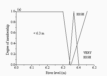 | 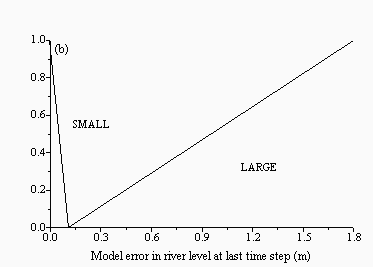 |
| Figure 3: Membership functions for the inputs: (a) current level and (b) model error at the last time step for the FBM for Skelton | |
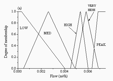 | 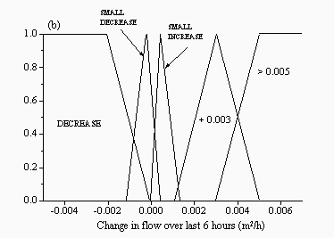 |
| Figure 4: Membership functions for the inputs: (a) current flow and (b) change in flow for the FMM for the Upper Wye | |
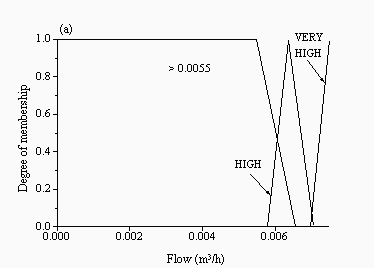 | 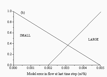 |
| Figure 5: Membership functions for the inputs: (a) current flow and (b) model error at the last time step for the FBM for the Upper Wye | |
FMM rules for Skelton are listed in Table 3. The FMM recommends the HNN model the majority of the time, but especially on the rising limb of the hydrograph at LOW to HIGH levels, where LOW to HIGH are the fuzzy sets shown in Figure 2a. The HNN model is also recommended on the falling limb some of the time. The SLFM predictor is only recommended on the rising limb of the hydrograph at HIGH and VERY HIGH levels, which suggests that it was able to characterise this portion of the hydrograph better than the other models. Naive predictions are recommended at the peaks of the hydrograph, when there is not much change, or where the water level is rising slightly. The ARMA model is recommended on the falling limb of the hydrograph and where there is a very steep rise in the water level over the 6 hour period.
 |
|
|
FMM rules for the Upper Wye are listed in Table 4. The 11 rules enclosed by the dark lines at the lower left corner of the rulebase did not fire during the original optimisation of this model, using 1985 data, nor with data from 1984. However, all rules fired when 1986 data were used, which reflects the fact that the 1986 data set is quite different from those of the other two years, and contains events not seen in either the training year or in 1984. Given these problems, no specific conclusions can be made about these rules, but the final arrangement of rules emerging from the genetic algorithm could have contributed to the higher overall error for 1986 that is listed in Table 8. For the other 14 rules, TOPMODEL is recommended on the falling limb at HIGH flows, and at LOW to MED flows when the change in flow is >0.005 m2/h. The rest of the time the NN1 and NN2 models are recommended. At LOW flows, and at a SMALL DECREASE in flow, the ARMA model is recommended. Neither the naive predictions nor the NN3 model is recommended in the set of 14 rules that fired during the optimisation process.
 |
|
|
Operational rules for the FBM approach are listed in Appendix I. These rules were not optimised with a genetic algorithm, but were instead formulated to reflect a crisp Bayesian approach in those situations where one model was clearly superior to the others, and a fuzzy Bayesian approach when several models were in contention for best performer. In the latter situation, the FBM can recommend any combination of models at the current time step, which results in a form of weighted average obtained from the best models in the previous time step. In this manner, the arbitrary boundary associated with choosing only the best model is fuzzified. FBM rules used for the Upper Wye were identical to those used for Skelton, although two extra rules were needed at each different level, in order to take all six models into account.
The individual models and the four integrating methods were assessed using one standard global goodness-of-fit statistic: root mean squared error. Results for each individual model were then divided into the percentage of predictions that occurred within 5, 10 and 25% of the observed (which included both over- and under-predictions). The global goodness-of-fit statistics are listed in Table 5. The best performing individual and multi-model approaches have been underlined. A breakdown into over- and under-predictions is provided in Table 6.
| Model | Approach | Training | Validation |
|---|---|---|---|
| HNN | Individual | 0.051 | 0.056 |
| ARMA | Individual | 0.082 | 0.098 |
| SLFM | Individual | 0.109 | 0.110 |
| Naive | Individual | 0.165 | 0.159 |
| Average | Multi-model | 0.087 | 0.086 |
| CBM | Multi-model | 0.041 | 0.042 |
| FMM | Multi-model | 0.045 | 0.048 |
| FBM | Multi-model | 0.038 | 0.040 |
For the individual models the global RMSE values indicate that the HNN model performed much better than the other three models on both the training and the validation datasets. Of the four multi-model approaches, the simple averaging model performed the poorest of the four approaches and produced a greater level of error than the individual HNN model. The patterns of residuals associated with the individual models did not therefore cancel each other out. The other three multi-model approaches, on the other hand, all produced better RMSE statistics than the HNN. FBM predictions had the lowest RMSE values.
The over- and under-predictions of the individual models indicate that the HNN had a fairly even distribution of under- and over-predictions while the ARMA, SLFM and naive estimates were consistently over-predicted. However, the total percentage of predictions within �5% of the observed is similar for each of the models. For the four integrating methods, there was a tendency towards overprediction although this was less prounounced for the CBM. The total percentage of predictions within �5% is again quite high and similar across the different methods. The CBM was correct 2.9% of the time on the training dataset and 2.3% of the time on the validation dataset, which are the remaining percentages that are unaccounted for in Table 6. For the other models, these percentages were negligible. This indicates that the best performing model at the last time step (t-1 hour) is not necessarily a good indication of which model to use at the current time step with a forecasting horizon of t+6 hours. However, the result for individual models was still very good since the majority of predictions were within �5% of observed. This could also go some way toward explaining why the FMM did not perform as well as the two Bayesian approaches in terms of the RMSE. Although specific model types were better suited to certain flow conditions, as indicated in the rulebase provided in Table 3, the river level behaviour at Skelton is perhaps not as homogenous as one might expect, given that the catchment does not respond that quickly at this location. However, the fuzzification of the Bayesian approach gave improved results, which in the worse case scenario should have approximated the CBM, but which benefitted from the option to recommend competing models.
| Model | Approach | Type of prediction | Training 5% | Validation 5% | Training 10% | Validation 10% | Training 25% | Validation 25% |
|---|---|---|---|---|---|---|---|---|
| HNN | Individual | under | 48.3 | 45.0 | 3.8 | 4.0 | 1.3 | 1.7 |
| over | 41.3 | 42.7 | 4.1 | 5.3 | 0.9 | 1.0 | ||
| ARMA | Individual | under | 15.2 | 16.3 | 4.0 | 3.2 | 2.7 | 2.8 |
| over | 72.7 | 72.4 | 4.8 | 4.8 | 0.4 | 0.3 | ||
| SLFM | Individual | under | 26.0 | 27.3 | 4.7 | 3.1 | 2.9 | 2.8 |
| over | 56.2 | 56.2 | 7.0 | 6.5 | 2.3 | 2.9 | ||
| Naive | Individual | under | 19.9 | 20.0 | 4.8 | 4.9 | 5.1 | 4.1 |
| over | 48.9 | 50.2 | 10.4 | 9.7 | 5.3 | 5.9 | ||
| Average | Multi-model | under | 21.1 | 21.1 | 3.8 | 3.0 | 2.8 | 2.7 |
| over | 67.2 | 67.2 | 4.2 | 4.8 | 0.6 | 0.6 | ||
| CBM | Multi-model | under | 39.4 | 38.5 | 1.8 | 1.9 | 0.8 | 1.3 |
| over | 53.8 | 54.8 | 1.0 | 1.0 | 0.1 | 0.3 | ||
| FMM | Multi-model | under | 20.2 | 19.2 | 2.2 | 2.0 | 1.1 | 1.5 |
| over | 74.3 | 75.3 | 2.0 | 1.8 | 0.1 | 0.2 | ||
| FBM | Multi-model | under | 26.9 | 24.8 | 2.1 | 2.2 | 0.9 | 1.2 |
| over | 69.2 | 70.9 | 0.7 | 0.5 | 0.1 | 0.1 |
Neither of these global evaluation measures provides any specific information about model performance at high levels, which in a flood forecasting context are of most importance. An additional evaluation criterion was therefore used in which model performance for predicting the timing of two operational alarm levels was determined. When water levels at Skelton reach 3m, standby alarms to duty officers monitoring the catchment are triggered. When the level reaches 3.5m, an area alert is activated. Then, as the level continues to rise, a series of different site specific operational instructions and warnings are issued. For the rising limb of all flood events, in both the training and the validation datasets, the percentage of times that a given model predicted the alarms earlier, at the correct hour, and later than the actual time at which the level was reached, was calculated. These results are listed in Table 7. For those flood events in which the standby and area alarms were predicted earlier or later than the actual times at which these levels were reached, the average number of hours that the prediction was early or late was also calculated, and this information is provided alongside the percentage figures in square brackets.
For the individual models, the naive predictions of the standby and the area alarm levels were always late, and by exactly 6 hours, as each prediction is simply a lagged version of the actual values. The ARMA models also always predicted the alarm levels late and even failed to predict one standby alarm in the validation dataset. However, the average hours late varied between 3.4 and 3.9, representing a 40% improvement over the naive predictions. The HNN model showed much better performance in predicting the time at which these alarm levels would be reached, with correct alarm predictions being produced more than 50% of the time on the validation dataset. There was also a more even distribution of late and early predictions, where an early prediction of 1 to 2 hours is less serious than a late one. The use of data at the original resolution of 15 minutes might have improved the timing of these predictions. For the multi-model approaches, the averaging method appears to have approximated an ARMA solution in terms of predicting the standby and alarm levels, which were predicted late almost 100% of the time. The average number of hours by which the predictions were late was also similar. The other multi-model solutions, however, were all closer in behaviour to the individual HNN model. This is not a surprising result since this model performed much better relative to the other individual models, especially when predicting the standby and alarm levels. It was also, doubtless, responsible for the dominance of the HNN in the multi-model predictions although the overall RMSE value obtained with the FBM approach, for example, was better.
| Model | Approach | Alarm | Early (T) | Early (V) | Correct (T) | Correct (V) | Late (T) | Late (V) |
|---|---|---|---|---|---|---|---|---|
| HNN | Individual | standby | 21 [1.0] | 30 [1.7] | 31 | 50 | 48 [1.0] | 20 [1.5] |
| area | 14 [1.3] | 14 [1.0] | 48 | 72 | 38 [1.9] | 14 [1.0] | ||
| ARMA | Individual | standby | 0 | 0 | 0 | 0 | 100 [3.4] | 90* [3.8] |
| area | 0 | 0 | 0 | 0 | 100 [3.6] | 100 [3.9] | ||
| SLFM | Individual | standby | 7 [2.5] | 10 [3.0] | 17 | 10 | 76 [3.5] | 80 [2.8] |
| area | 0 | 0 | 10 | 29 | 90 [2.7] | 71 [3.2] | ||
| Naive | Individual | standby | 0 | 0 | 0 | 0 | 100 [6.0] | 100 [6.0] |
| area | 0 | 0 | 0 | 0 | 100 [6.0] | 100 [6.0] | ||
| Average | Multi-model | standby | 0 | 0 | 0 | 10 | 100 [3.2] | 90 [3.1] |
| area | 0 | 0 | 0 | 0 | 100 [3.4] | 100 [3.6] | ||
| CBM | Multi-model | standby | 21 [1.0] | 20 [2.0] | 28 | 50 | 52 [1.1] | 30 [1.7] |
| area | 10 [1.0] | 14 [1.0] | 43 | 57 | 47 [1.6] | 29 [2.0] | ||
| FMM | Multi-model | standby | 17 [1.0] | 30 [1.3] | 24 | 50 | 59 [1.1] | 20 [1.5] |
| area | 10 [1.5] | 14 [1.0] | 43 | 57 | 47 [1.7] | 29 [1.5] | ||
| FBM | Multi-model | standby | 17 [1.0] | 30 [1.3] | 31 | 50 | 52 [1.1] | 20 [1.5] |
| area | 9 [1.0] | 14 [1.0] | 48 | 57 | 43 [1.6] | 29 [1.5] |
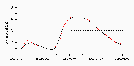
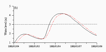
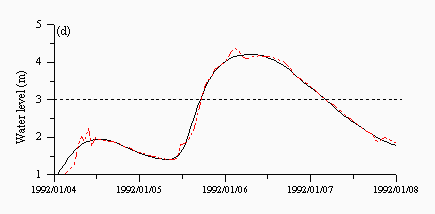
Figures 6 and 7 are plots of a storm event in January 1992 taken from the validation dataset. A dotted line is drawn at a level of 3m, which is the level of the standby alarm. The HNN model (Figure 6a) shows the best performance, predicting both alarm levels well. The naive predictions in Figure 6c clearly show the six hour lag at each prediction point while the ARMA model in Figure 6b shows a better performance but predicts the standby and area alerts late in both events. Finally, the SLFM in Figure 6d appears to show a combination of different responses and predicts both alarm levels late. It does however appear to predict the falling limb much better than any other aspect of the hydrograph.
 |  |
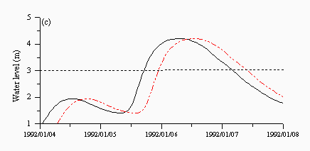 | 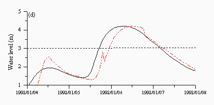 |
| Figure 6: Individual predictions from the (a) hybrid neural network (b) ARMA (c) naive and (d) SLFM predictors for a flood event in January 1992. The black lines are the observed and the red lines are the predicted. | |
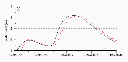
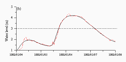
For the multi-model approaches, the averaging model (Figure 7a) shows a lag time pattern, which is reflected in Table 7. The other three multi-model approaches produced results which were similar to the HNN, which is understandable, given the preference of the other solutions to select the HNN model. Moreover, the HNN model probably performs well enough that it might be used in isolation. However, the multi-model approaches did result in overall improvements that might be reflected in other aspects of the hydrograph and which might, therefore, be relevant to other forecasting purposes such as drought monitoring and reservoir management. Another important consideration is the catchment response. This research and testing exercise was based on Skelton which has a relatively stable regime. It is interesting to see how the different methods perform on flashier catchments such as the Upper Wye, which are provided in the next section, where no single method will be seen to dominate.
 |  |
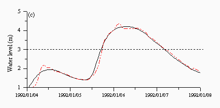 |  |
| Figure 7: Predictions from the (a) average (b) CBM (c) FMM and (d) FBM approaches for a flood event in January 1992. The black lines are the observed and the red lines are the predicted. | |
When both global and storm-specific evaluation measures are taken into account, the individual HNN model and the FBM predictor appear to perform the best of all the approaches, although the FBM performed better overall. There were no RFFS benchmarks against which these results could be compared. However, the results are extremely good and the best models closely match the rise and fall of the hydrograph. If these results can be consistently reproduced for a range of real-world flood events, at a number of different sites and scales, then there would be little doubt about the utility of this method as a practical flood prediction tool.
The individual models and the four integrating methods developed for the Upper Wye were also evaluated on a global basis using root mean squared error and the percentage of predictions that occurred within 5, 10 and 25% of the observed (which included both over- and under-predictions). The global goodness-of-fit statistics are listed in Table 8 and a breakdown into over- and under-predictions is provided in Table 9. Table 10 also provides the % of predictions greater than 25% of observed (regardless of whether these are over- or under-predictions) and the % correct, since both of these values were significant for certain models, which was not the case for Skelton. It is not possible to make a direct comparison between the Skelton and the Upper River Wye statistics because the first relates to level data in m and the other is flow data in m3/h. However, RMSE does allow for a comparison of the different model types at a given station, and visual inspection of a typical flood event provides a good comparison of the ability of the models at both stations to predict the rise and fall of the hydrograph, the latter being the most important measure of evaluation for many practical applications.
| Model | Approach | 1984 | 1985 | 1986 |
|---|---|---|---|---|
| TOPMODEL | Individual | 1.518 | 1.417 | 1.182 |
| NN1 | Individual | 0.727 | 0.458 | 0.892 |
| NN2 | Individual | 0.557 | 0.515 | 0.877 |
| NN3 | Individual | 0.557 | 0.556 | 0.936 |
| ARMA | Individual | 0.599 | 0.602 | 0.817 |
| Naive | Individual | 0.594 | 0.797 | 1.140 |
| Average | Multi-model | 0.446 | 0.498 | 0.763 |
| CBM | Multi-model | 0.609 | 0.566 | 0.787 |
| FMM | Multi-model | 0.622 | 0.410 | 0.829 |
| FBM | Multi-model | 0.375 | 0.341 | 0.544 |
For the individual models, the global RMSE values indicate that the NN2 model has the lowest training error and produced the best generalisation for 1984 data (matching the 1984 performance of the NN3 model) while the ARMA model produced the best generalisation for 1986 data. Of the four integrating methods, the FBM performed the best overall, and the averaging model was the second best multi-model performer. Thus, for this station and this dataset, the patterns of residuals of the individual models have to some degree cancelled each other out and produced a better averaging than was the case with Skelton.
The over- and under-predictions of the individual models listed in Tables 9 and 10 exhibit considerable between-model variation. For TOPMODEL and each of the neural network solutions, a large percentage of predictions were greater than 25% although the figure for 1985 was lower for each neural network, which is to be expected since this was the training year. This is in contrast to Skelton where there was a negligible percentage of predictions greater than 25%, reflecting the more stable regime. The ARMA model and naive predictions, on the other hand, had about one third of the predictions correct, and a large percentage were within 5%. The similarities in percentage correct for the ARMA model and the naive predictions suggest that there were many situations of either low flow, or times with little change, which both models were able to handle better than any of the other individual models. For the four integrating methods, the percentage of predictions within 5% of observed was higher than either TOPMODEL or the individual neural networks, and the percentage of predictions greater than 25% was also lower, indicating general improvements in performance. However, the ARMA and naive predictions were still substantially better in the lower flow areas so the improvements in performance that were made by the multi-model approaches were probably gained at the higher flows, which in a flood forecasting context is the most important feature. The CBM, on the other hand, was the only method that was able to take direct advantage of the ability of the naive and ARMA models to predict these areas of low flow or little change perfectly; this was reflected in the figures for % correct, which were similar in all three methods.
| Model | Approach | Type of prediction | 1984 | 1985 5% | 1986 | 1984 | 1985 10% | 1986 | 1984 | 1985 25% | 1986 |
|---|---|---|---|---|---|---|---|---|---|---|---|
| TOPMODEL | Individual | under | 1.8 | 5.3 | 6.3 | 2.8 | 5.4 | 8.9 | 11.2 | 19.4 | 30.6 |
| over | 1.5 | 4.7 | 4.4 | 1.5 | 3.4 | 3.4 | 3.1 | 4.8 | 4.9 | ||
| NN1 | Individual | under | 10.3 | 14.6 | 12.7 | 13.3 | 17.0 | 14.2 | 16.7 | 13.2 | 13.1 |
| over | 6.4 | 12.6 | 10.3 | 3.3 | 7.6 | 6.7 | 5.5 | 12.8 | 10.5 | ||
| NN2 | Individual | under | 11.4 | 13.8 | 13.6 | 16.9 | 19.3 | 15.8 | 7.8 | 5.7 | 5.5 |
| over | 9.9 | 12.2 | 11.6 | 3.8 | 10.6 | 8.7 | 5.9 | 14.8 | 9.9 | ||
| NN3 | Individual | under | 13.6 | 14.1 | 12.0 | 15.8 | 16.6 | 14.2 | 5.5 | 7.6 | 8.6 |
| over | 11.6 | 12.1 | 11.0 | 8.7 | 8.3 | 7.1 | 9.9 | 14.2 | 10.7 | ||
| ARMA | Individual | under | 12.9 | 18.2 | 15.6 | 7.3 | 3.8 | 4.0 | 5.3 | 3.0 | 3.0 |
| over | 28.6 | 39.4 | 36.6 | 7.2 | 4.7 | 4.4 | 4.5 | 1.7 | 2.1 | ||
| Naive | Individual | under | 7.7 | 6.9 | 6.5 | 5.9 | 3.7 | 3.1 | 5.7 | 3.6 | 3.7 |
| over | 34.5 | 36.8 | 32.7 | 8.2 | 8.0 | 7.9 | 5.2 | 3.4 | 4.0 | ||
| Average | Multi-model | under | 12.8 | 22.3 | 20.4 | 17.0 | 19.3 | 15.1 | 7.8 | 6.0 | 5.3 |
| over | 9.1 | 16.3 | 14.2 | 5.6 | 9.7 | 8.9 | 7.7 | 12.0 | 10.5 | ||
| CBM | Multi-model | under | 15.6 | 17.4 | 15.6 | 4.7 | 4.2 | 4.6 | 3.0 | 2.9 | 3.0 |
| over | 29.8 | 34.1 | 30.0 | 4.9 | 4.7 | 4.8 | 2.3 | 1.9 | 2.3 | ||
| FMM | Multi-model | under | 28.2 | 31.6 | 27.3 | 3.8 | 4.0 | 4.4 | 3.1 | 2.2 | 2.4 |
| over | 12.8 | 28.2 | 24.4 | 4.8 | 11.3 | 8.5 | 7.0 | 11.6 | 12.6 | ||
| FBM | Multi-model | under | 14.5 | 23.1 | 21.1 | 17.3 | 18.9 | 15.1 | 6.0 | 4.7 | 4.5 |
| over | 10.3 | 17.9 | 15.3 | 5.7 | 10.0 | 8.8 | 6.6 | 11.9 | 10.4 |
| Model | Approach | 1984 | 1985 > 25% | 1986 | 1984 | 1985 %correct | 1986 |
|---|---|---|---|---|---|---|---|
| TOPMODEL | Individual | 77.8 | 56.6 | 41.1 | 0.3 | 0.5 | 0.5 |
| NN1 | Individual | 43.4 | 20.5 | 31.3 | 1.1 | 1.7 | 1.2 |
| NN2 | Individual | 43.4 | 22.3 | 33.5 | 0.8 | 1.3 | 1.4 |
| NN3 | Individual | 33.5 | 25.8 | 34.9 | 1.4 | 1.3 | 1.5 |
| ARMA | Individual | 4.5 | 1.2 | 1.4 | 29.7 | 28.1 | 32.9 |
| Naive | Individual | 3.5 | 2.3 | 2.6 | 29.3 | 35.3 | 39.6 |
| Average | Multi-model | 39.0 | 11.6 | 23.9 | 1.1 | 2.9 | 1.7 |
| CBM | Multi-model | 1.6 | 1.3 | 1.6 | 38.1 | 33.5 | 38.1 |
| FMM | Multi-model | 37.4 | 5.5 | 16.4 | 3.0 | 5.7 | 4.1 |
| FBM | Multi-model | 38.5 | 10.5 | 23.1 | 1.1 | 3.1 | 1.8 |
Once again, neither of these global evaluation measures provides information about the performance of these models at higher flows. Since there were no operational definitions on which to base flood specific evaluation measures, the ability to predict the peak of each flood event was evaluated. Table 11 lists the percentage of peak predictions that were early, on time or late for all flood events, along with the average number of hours early or late, which are again provided alongside the percentage figures in square brackets.
Looking at the individual model results, the naive predictions for the flood events were always one hour late, which is to be expected since these are simply the original observations lagged by one hour. Most of the time the ARMA model also predicted the flood events late, with an average lag time of one hour. Each of the neural networks produced a larger percentage of correct peak predictions than the naive and ARMA models, while TOPMODEL predictions were the poorest of the individual models, with average late predictions for 1985 and 1986 being greater than the one hour forecasting horizon. For the multi-model approaches, both averaging and CBM methods predicted the correct time of peak less often than the neural networks but more frequently than the ARMA or naive models. The FMM and FBM methods both gave better time of peak prediction, especially for 1985 and 1986. Overall, similar average lag times were obtained for the individual and multi-model approaches, with peak lateness not usually exceeding the forecasting horizon of one hour. Several of the 1984 predictions were however, more than one hour early.
| Model | Approach | 1984 | 1985 Early | 1986 | 1984 | 1985 On time | 1986 | 1984 | 1985 Late | 1986 |
|---|---|---|---|---|---|---|---|---|---|---|
| TOPMODEL | Individual | 100 [2.0] | 37 [1.0] | 16 [1.0] | 0 | 37 | 42 | 0 | 26 [1.5] | 42 [2.0] |
| NN1 | Individual | 29 [2.0] | 0 | 14 [1.0] | 57 | 56 | 41 | 14 [1.0] | 44 [1.0] | 45 [1.0] |
| NN2 | Individual | 29 [2.0] | 0 | 14 [1.0] | 71 | 67 | 32 | 0 | 33 [1.0] | 54 [1.0] |
| NN3 | Individual | 29 [1.5] | 0 | 14 [1.0] | 71 | 67 | 36 | 0 | 33 [1.0] | 50 [1.0] |
| ARMA | Individual | 0 | 0 | 9 [1.0] | 29 | 44 | 27 | 71 [1.0] | 56 [1.0] | 64 [1.0] |
| Naive | Individual | 0 | 0 | 0 | 0 | 0 | 0 | 100 [1.0] | 100 [1.0] | 100 [1.0] |
| Average | Multi-model | 29 [1.5] | 0 | 4 [1.0] | 42 | 44 | 32 | 29 [1.0] | 56 [1.0] | 64 [1.0] |
| CBM | Multi-model | 14 [2.0] | 0 | 9 [1.0] | 43 | 33 | 32 | 43 [1.0] | 67 [1.0] | 59 [1.0] |
| FMM | Multi-model | 29 [2.0] | 0 | 14 [1.0] | 57 | 67 | 45 | 14 [1.0] | 33 [1.0] | 41 [1.0] |
| FBM | Multi-model | 14 [2.0] | 0 | 14 [1.0] | 72 | 67 | 45 | 14 [1.0] | 33 [1.0] | 41 [1.0] |
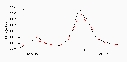
Figures 8 and 9 are plots of a flood event taken from 1986, which is the validation year characterised by more high flow events. TOPMODEL predictions are quite good and predict the peak of the hydrograph well albeit one hour late (Figure 8a). Each of the neural networks underpredicts the peak, although the rising and falling limbs are predicted quite well (Figures 8b-d), while both the ARMA model (Figure 8e) and naive predictions (Figure 8f) clearly show a lag in the majority of the hydrograph, although this behaviour is more prounounced in the naive predictions than the ARMA model.
 |  |
 |  |
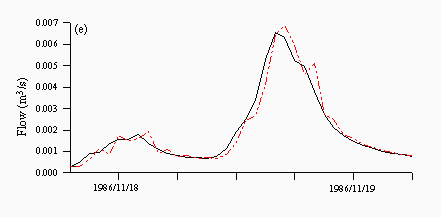 | 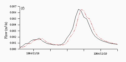 |
| Figure 8: Individual predictions from the (a) TOPMODEL (b) NN1 (c) NN2 (d) NN3 (e) ARMA and (f) naive predictors for a flood event in November 1986. The black lines are the observed and the red lines are the predicted. | |
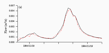
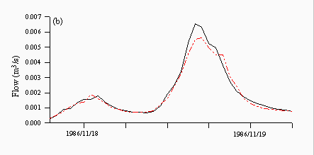
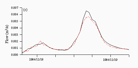
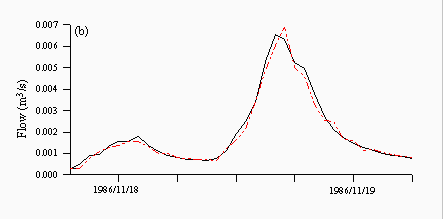
For the multi-model approaches, both the averaging model (Figure 9a) and the FMM (Figure 9c) underpredict the peak, while the CBM (Figure 9b) overpredicts the peak. However, the FBM output (Figure 9d), clearly matches all aspects of the hydrograph in a better manner than any of the other approaches, which therefore provides visual confirmation of the earlier statistical results.
 |  |
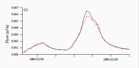 | 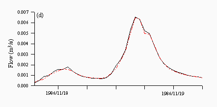 |
| Figure 9: Predictions from the (a) average (b) CBM (c) FMM and (d) FBM approaches for a flood event in November 1986. The black lines are the observed and the red lines are the predicted. | |
When both global and peak-specific evaluation measures are taken into account, the FBM is the best performer and appears to be well suited to predicting flashy types of behaviour, although this finding relates at present to the short forecasting horizons used in this exercise. Extending the forecasting horizon beyond the conventional one-step-ahead hourly prediction is the subject of future research.
This paper presented four different methodologies for integrating conventional and AI-based methods to provide a hybridised solution to the continuous river flow and flood forecasting problem. Individual models ranging from neural networks to statistical predictors were developed on a standalone basis for the River Ouse at Skelton and the Upper River Wye. A simple fuzzy logic model for Skelton and TOPMODEL predictions for the Upper Wye were also incorporated as additional model inputs. Each of these individual models were then integrated via Bayesian and fuzzy logic techniques. The addition of the fuzzy logic to the crisp Bayesian model yielded overall results that were superior to the other multi-model and individual approaches although this was more apparent for the Upper River Wye than for the River Ouse at Skelton. Moreover, the simplicity of the multi-model approaches equates to fast and inexpensive model development. However, both methods still require extensive testing on a wider range of stations types and catchments to determine their potential for operational flood forecasting and for other purposes which utilise continuous river level or river flow predictions. An important aspect of further testing should be the integration of these types of methods directly into a real-time operational forecasting and monitoring system. The best combination of models would appear to be naive, ARMA, possibly a SLFM and a neural network, integrated via a FBM approach. There is nothing to prevent this type of approach being incorporated into a PC-based system that is able to be run alongside whatever existing systems are currently in use. Only then, can the real practical benefits of this type of applied research be felt, which goes one step beyond the various types of academic exercise that are now being reported in the literature.
Abrahart, R.J. 1998. "Neural networks and the problem of accumulated error: an embedded solution that offers new opportunities for modelling and testing". Proceedings Hydroinformatics'98: Third International Conference on Hydroinformatics, Copenhagen, Denmark, 24-26 August 1998.
Abrahart, R.J. and Kneale, P.E. 1997. "Exploring Neural Network Rainfall-Runoff Modelling". Proceedings Sixth National Hydrology Symposium, University of Salford, 15-18 September 1997, 9.35-9.44.
Abrahart, R.J. and See, L. 1998. "Neural Network vs. ARMA Modelling: constructing benchmark case studies of river flow prediction". Proceedings GeoComputation'98: Third International Conference on GeoComputation, University of Bristol, United Kingdom, 17-19 September 1998.
Abrahart, R.J., See, L. and Kneale, P. 1998. "New tools for neurohydrologists: using 'network pruning' and 'model breeding' algorithms to discover optimum inputs and architectures". Proceedings GeoComputation'98: Third International Conference on GeoComputation, University of Bristol, United Kingdom, 17-19 September 1998.
Bathurst, J. 1986. "Sensitivity analysis of the Systeme Hydrologique Europeen for an upland catchment", Journal of Hydrology, 87, 103-123.
Beven, K.J., Kirkby, M.J., Schofield, N. and Tagg, A.F. 1984. "Testing a physically-based flood forecasting model (TOPMODEL) for three U.K. catchments", Journal of Hydrology, 69, 119-143.
Dougherty, M.S. 1997. "Meta-analysis of various short term load forecasts". Presented at the Engineering Applications of Neural Networks Conference, Stockholm, June 1997.
French, M.N., Krajewski, W.F. and Cuykendall, R.R. 1992. "Rainfall forecasting in space and time using a neural network", Journal of Hydrology, 137, 1-31.
Hsu, K-L, Gupta, H.V. and Sorooshian, S. 1995. "Artificial neural network modeling of the rainfall-runoff process", Water Resources Research, 31, 10, 2517-2530.
Karunanithi, N., Grenney, W.J., Whitley, D. and Bovee, K. 1994. "Neural Networks for River Flow Prediction", Journal of Computing in Civil Engineering, 8, 2, 201-220.
Kohonen, T. 1995. Self-Organizing Maps. Heidelberg: Springer-Verlag.
Knapp, B.J. 1970. Patterns of water movement on a steep upland hillside, Plynlimont, central Wales, Unpublished PhD Thesis, Department of Geography, University of Reading, Reading.
Minns, A.W. and Hall, M.J. 1996. "Artificial neutral networks as rainfall-runoff models", Hydrological Sciences Journal, 41, 3, 399-417.
Newson, M.D. 1976. The physiography, deposits and vegetation of the Plynlimon catchments, Institute of Hydrology, Wallingford, Oxon. Report No. 30.
Openshaw, S., Kneale, P., Corne, S. and See, L. 1998. The Feasibility of Neural Networks for Flood Forecasting. Final Report. MAFF Project OCS967P. School of Geography, University of Leeds.
Openshaw, S. and Openshaw, C. 1997. Artificial Intelligence in Geography. Chichester: John Wiley & Sons Ltd.
Quinn, P. F. and Beven, K. J. 1993. "Spatial and temporal predictions of soil moisture dynamics, runoff, variable source areas and evapotranspiration for Plynlimon, Mid-Wales", Hydrological Processes, 7, 425-448.
Raman, H. and Sunilkumar, N. 1995. "Multivariate modelling of water resources time series using artificial neural networks", Hydrological Sciences Journal, 40, 2, 145-163.
See, L. and Openshaw, S. 1998. " Using soft computing techniques to enchance flood forecasting on the River Ouse". Proceedings Hydroinformatics'98: Third International Conference on Hydroinformatics, Copenhagen, Denmark, 24-26 August 1998.
Smith, J. and Eli, R.N. 1995. "Neural-Network Models of Rainfall-Runoff Process", Journal of Water Resources Planning and Management, 121, 6, 499-509.
If the current level is LOW and
If the current level is MED and
If the current level is HIGH and
Similarly, the FBM rulebase for the Upper Wye can be given as:
If the current level is LOW and
If the current level is MED and
If the current level is HIGH and
| ARMA | = Autoregressive Moving Average Model |
| CBM | = Crisp Bayesian Model |
| FBM | = Fuzzy Bayesian Model |
| FMM | = Fuzzy Master Model |
| HNN | = Hybrid Neural Network |
| NN1 | = Original Neural Networks (24:12:12:1) |
| NN2 | = NN1 after magnitude based pruning |
| NN3 | = NN1 after skeletonization |
| SLFM | = Simple Linguistic Fuzzy Model |
| SOM | = Self Organizing Map |