Combining Physical
Indicators of
Brian Irvine, Jianhui Jin, Mike Kirkby, Andy Turner
Introduction
This poster shows indicators of physical land degradation
associated with soil erosion and salinity.
We are exploring how to combine these and other land degradation
indicators to produce synoptic predictions of the associated risks under
different environmental change scenarios.
Land degradation and desertification are processes characterised by deterioration in the quality of land in terms of its capability to support land uses, flora and fauna. Desertification is extreme land degradation where land loses much of its natural productivity, usually associated with sparse vegetation of low biodiversity. As the soil becomes prone to erosion vegetation becomes less likely to grow back in a positive feedback loop. Usually the extremes are associated with regional and climatic trends which may threaten large areas. In the Mediterranean climate region of the Europe Union (EU) these processes have been of concern for well over a decade. In this region it is thought that climate change compounded by changing land use is resulting in natural resources (especially water) being used unsustainably, increasing both the incidence and risk of land degradation.
Some areas are more likely to degrade than others and in different ways. In some areas land degradation has been observed for some time and no mitigation action has been taken, in other areas something has been done to try and alleviate certain problems and reduce the risks. This poster does not try to prescribe what should be done or where mitigation is a priority, it merely illustrates an attempt to map out the risks.
Since the early 1990s there have been numerous European
Commission (EC) funded research projects that have investigated land
degradation. The process is now known to
be complex, socio-economics is intricately interrelated and all the various
factors interact at different spatial and temporal scales. This poster is a product of some work which
is trying to draw it all together and focus on the EU. It is a combined effort of three EC funded
projects: DESERTLINKS1, MEDACTION2, and PESERA3.
Erosion Risk
Since the early 1990s, erosion risk models and indicators
have been developed through successive EC funded research projects. The Regional Desertification Indicator (RDI),
which has been expanded in the Pan-European Soil Erosion Assessment (PESERA3),
offers a methodology to assess regional soil erosion risk. The RDI is based on
concepts developed in MEDALUS4 and offers an explicit theoretical
response based on a simple and conservative soil erosion model. The model makes use of land-use, topographic
soil and climatic data (Table 1).
Table 1: Data requirements for the implementation of the
PESERA_RDI model at 1km
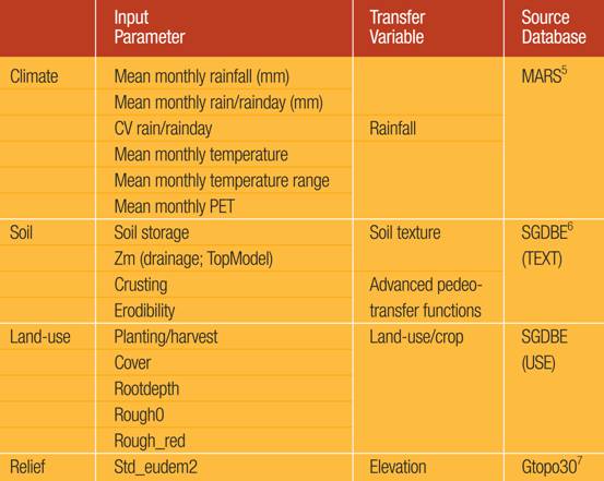 NB:
drainable pore space and available water content to be provided at 1km scale
(bulk density, texture, organic matter)
NB:
drainable pore space and available water content to be provided at 1km scale
(bulk density, texture, organic matter)
The RDI model combines ground cover, surface crusting,
runoff and sediment transport, to give an estimate of water and sediment
delivered to stream channels. A model
schematic is shown in Figure 1. Modelled
erosion risk is consistent with finer scale erosion models for flow strips, and
is integrated across the frequency distribution of storm magnitudes (Figure 2). The model partitions daily precipitation into
Hortonian and saturation overland flow, subsurface
flow and evapo-transpiration. Hortonian overland
flow, which is mainly responsible for soil erosion, is generated with respect
to local soil and sub-surface moisture characteristics. The emphasis of the PESERA-RDI model is the
prediction of hillslope erosion, and the delivery of
erosion products to the base of each hillslope. Channel delivery processes and channel
routing are explicitly not considered.
Figure 1: PESERA Model
Schematic
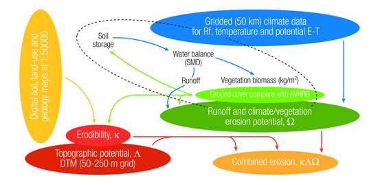
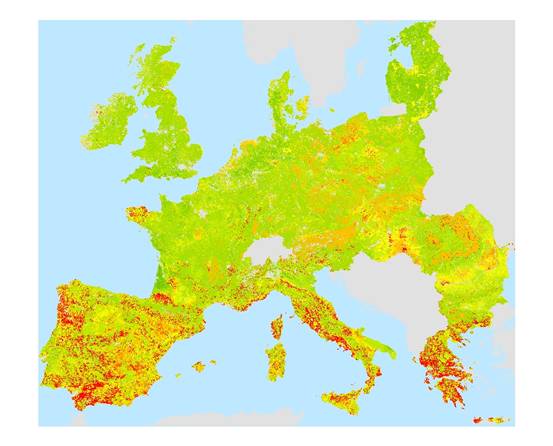
Figure 2: Map Of Erosion Estimate Surface
The physical basis of the RDI
model offers the potential to enhance future land degradation predictions,
distinguishing between the effects of land-use and climatic changes. As these
components are explicit within the model, the sensitivity of changing
environments can be explored directly.
Although currently being applied at a 1 km resolution for
Although available on a Pan-European scale the, 1km data
resolution is coarse when considering the local scale and more refined data is
desirable. Local data sets offer higher
resolution than that applied at the European scale.
Salinisation Risk
Soil salinisation is a process through which soil becomes more saline. This can happen in at least three ways:
- Soil near the surface can become more saline as salts are drawn up in solution from water within the soil and bedrock.
- Coastal flooding can cause salinisation by an influx of salt water.
- Irrigation with slightly saline water in a way that resulting evapo-transpiration leads to an accumulation of saline deposits.
In general, the more saline a soil, the more limited the vegetation that it supports. Some vegetation grows better on slightly saline soils, though there are limits beyond which vegetation dies back. If a soil is gradually becoming more saline but is likely only to reach a level of salinity at which much of the present ecosystem will persist, then arguably this does not pose a major land degradation risk. On the other hand, if there is a likelihood of salinisation continuing unchecked, or if it is unlikely that the present ecosystem will cope, then arguably there is a high land degradation risk.
Salinised soils can be treated by leaching (flushing with water) and by adding neutralisers to the soil. This is a remedy for cultivated land that has become salinised, but is also a way of preparing uncultivated land for production. Salinised land varies in how easily and inexpensively it can be treated. Thus, in some areas land is more likely to be treated and in others it is likely to be abandoned or left unused.
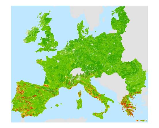
Figures 3 and 4 are maps of predicted salinisation surfaces at a 1km resolution. The maps were generated using available data and are based on some simplifying assumptions. Equation 1 is the formula applied to combine three variables PM, FLUX and STDEVEL into salinity estimates.
Equation 1: Salinity
Estimation Formula
SALINITY = ( ( 0.1 + PM ) * FLUX ) / ( 10 + STDEVEL )
PM is a parent material variable. This is a simple bi-valued parent material classification based on source SGDE data6. Each 1km region was coded 1 if the main parent material could potentially break down into salts and 0 otherwise.
FLUX is a proxy for soil water level fluctuation derived from MARS data5. For Figure 3 FLUX was calculated as follows: The water balance for each month was calculated as rainfall minus potential evapo-transpiration (PET). Then the FLUX was taken as the minimum of; the maximum water balance, and the negative of the minimum water balance for the 12 monthly values. For Figure 4 PET was simply substituted for FLUX. The variable FLUX is responsible for the difference in the surfaces mapped in Figures 3 and 4.
STDEVEL is the standard deviation of elevation as calculated from source GTOPO30 data7. The source data was projected and transformed into a 1km resolution grid to align with the other data. From this, the standard deviation of elevation for each cell and its 8 immediate neighbours was calculated. Thus, flatter areas attained a lower value and therefore by Equation 1 a higher estimate of salinisation.
Figure 3: Map Of Estimated Natural Salinisation
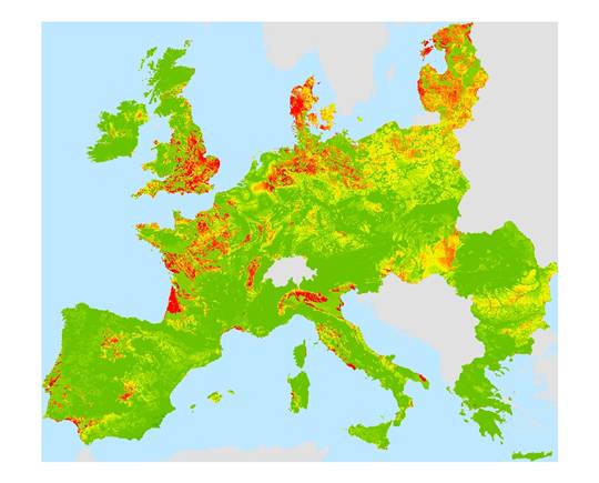
Figure 4: Map Of Estimated Secondary Salinisation
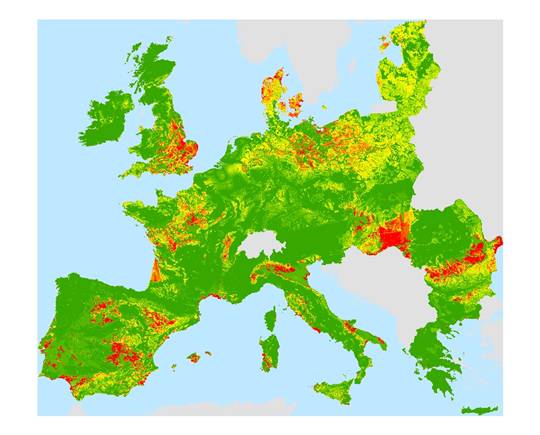
Figure 3 shows where soils are more likely to be saline
naturally especially in southern
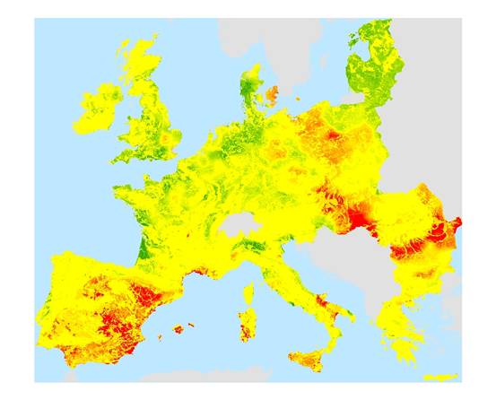
Figure 5 is a map of Z-scores of secondary salinity minus Z-scores of natural salinity. This map is interesting as arguably it is a better indicator of land degradation risk from soil salinisation than Figures 3 and 4. The reasoning is that areas that are likely to be naturally saline are more likely to contain ecosystems that can cope, whereas areas which are not naturally saline (but have the potential to be) are more likely to have been irrigated to produce crops and more likely to be recognised as good quality agricultural areas and thus at risk of degradation.
Figure 5: Map Of The Difference Between Secondary And Natural Salinisation Z-scores
Attempting to combine and interpret land degradation indicators is important for our understanding of land degradation processes and for our forecasting of what might be the general effects of environmental change. Combining different indicators is challenging. How can it be done in a way which is both meaningful and unbiased? Here are two different approaches of combining land degradation risk indicators. One is based on using the Z-scores of each indicator, and the other is based on fuzzy logic.
Z-score Approach
A difficulty in combining land degradation indicators is that their value ranges and distributions are often very different. One way to overcome this is to firstly transform each indicator into a Z-score. The Z-scores are more comparable and more easily combined using a simple formula (e.g. adding). Converting to Z-scores has the effect of transforming the original distribution of a variable to one with a mean of zero and standard deviation of one. A Z-score quantifies the original value in terms of the number of standard deviations that the value is from the mean of the distribution. Equation 2 is the formula for converting an original value into a Z-score.
Equation 2: For Calculating
Z-scores
Z-score = ( value – mean ) / ( stddev )
mean is the mean of all values
stddev is the standard deviation of all values
Figure 6 below is a map of a surface generated by adding the Z-scores of the Erosion surface depicted in Figure 2 with those of the Salinisation Risk surface depicted in Figure 5.
Figure 6: Land
Degradation Risk Map Generated by Combining Erosion Surface and Salinisation Risk Surface Using Z-scores
Fuzzy Modelling
Approach
Fuzzy modelling provides another way of combining variables into land degradation risk surfaces. There are three components to a fuzzy model:
- A set of membership functions, which define the degrees of membership of values to fuzzy sets;
- A rule base, which is a collection of fuzzy IF-THEN rules; and,
- A fuzzy inference engine that drives the model by execution of the rule base in response to a set of fuzzy inputs
From the ranges of the erosion estimates and the salinity risk surfaces shown in Figures 2 and 5 respectively, the membership functions depicted at the top of Figure 7 were defined. Along the X-axes of these membership functions are the values for each variable and the Y-axis scales the degree of membership from zero at the intersection of the X-axis to one above. It can be seen that every erosion estimate has a non-zero degree of membership for all values in the range [0, 30], for salinity risk values in the range [0, 5] belong to all three fuzzy classes (low, medium and high) to some degree. The five rules in Figure 7 constitute the rule base and the entire diagram illustrates how a pair of input values are parsed by each rule and how the result of this are combined and defuzzified into a land degradation risk value. It should be noted that this is but one way of performing fuzzy inference and that there are a number of alternatives. Also, fuzzy inference is usually used in far more complex circumstances with many more rules and more complex membership functions.
Figure 7: Fuzzy Inference
Diagram
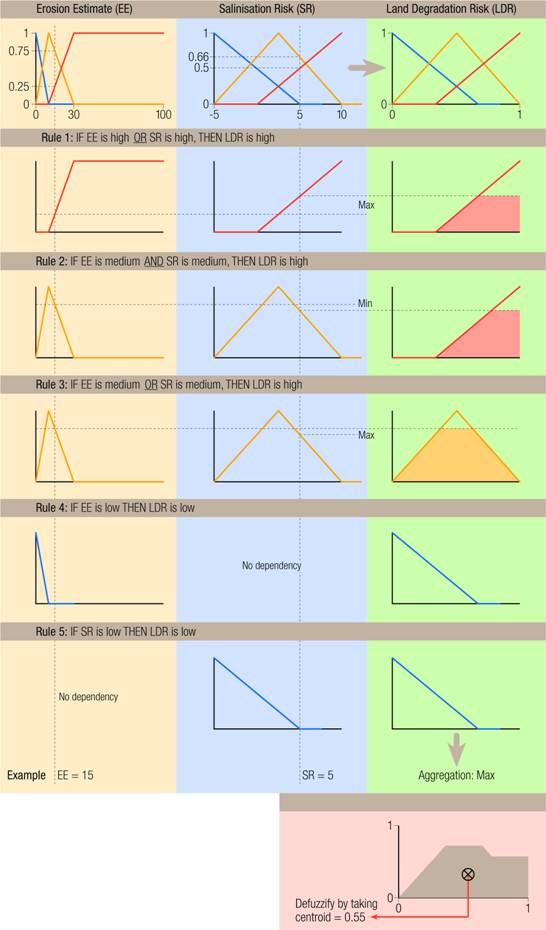
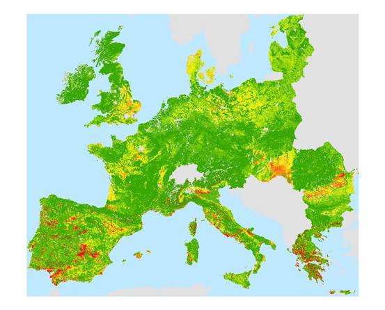
Figure 8 is a map of the resulting land degradation risk surface. It has a similar pattern to the surface depicted in Figure 6, though the maps look different at a glance.
Figure 8: Land
Degradation Risk Map Generated by Combining Erosion Surface and Salinisation Risk Surface Using Fuzzy Inference
Further Points
The erosion surface shown in Figure 3 uses land use as an input and is really an estimate of how much eroded material there is likely to be for a given 1km cell. Arguably, Figure 3 does not show the likely effects of erosion in terms of land degradation risk and that to do this some further translation is needed.
The salinity risk maps (Figures 3 and 4) were based expert opinion coded as a mathematical equation. A fuzzy model could have been employed instead. I this way a salinity based land degradation risk indicator could have been generated in a single step.
It has been reasoned that the simplifying assumptions made in the generation of the surface depicted in Figure 5 are appropriate, but the assumption may be flawed. Nonetheless some further analysis of the salinity surfaces should be done. Are the combined land degradation risk indicators depicted in Figures 6 and 8 broadly correct? Perhaps the next step is to collate feedback and do some more detailed work in case study areas.
There is a need to produce estimates of land degradation risks under different environmental change scenarios and incorporate socio-economics in a more integrated way. Arguably, the difference between land degradation risk estimates under different environmental change scenarios is what is most interesting.
References
1. DESERTLINKS home page URL:
http://www.kcl.ac.uk/kis/schools/hums/geog/desertlinks/
2. PESERA home page URL:
http://pesera.jrc.it
3. MEDACTION home page URL:
http://www.icis.unimaas.nl/medaction/
4. MEDALUS home page URL:
http://www.medalus.demon.co.uk/
5. Monitoring Agriculture with Remote Sensing (MARS)
http://mars.jrc.it/
6. The Soils Geographic Database of Europe version
3.2.8.0 (SGDE)
http://data-dist.jrc.it/eu4u/soilmap.html
7. GTOPO30 Global Topography Data home page URL:
http://edcdaac.usgs.gov/gtopo30/gtopo30.html
Acknowledgements
This work was supported by the following European Commission
grants:
QLKS-CT-1999-01323 (PESERA)
EVK2-CT-2000-00085 (MEDACTION)
EVK2-CT-2001-00109 (DESERTLINKS)
Thanks to the Graphics Unit in the