Spatial Interaction Modelling: Core ideas
[Practical 4 of 11 - Part 2]
Getting the Data:
The previous part of the practical built up a framework of comments to allow us to think about the bits we need to complete in order for this model to run. The first thing we need to do is get some data.
Because we are building a very basic model at the moment we are going to get the data and access it in a very basic way. We are going to create some data arrays with the data in. In a real world situation we would want to be able to read data in from a file or a series of files, that will come later in the course first we need to make sure we can run our model.
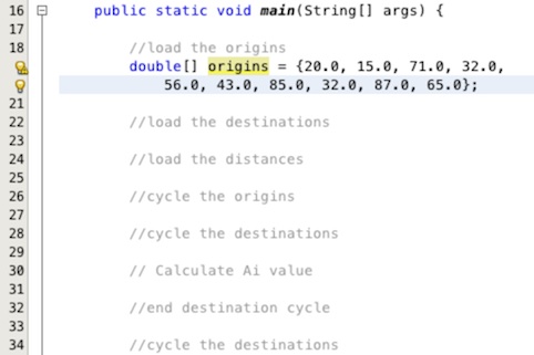
To create the origins data type the line double[] origins = {20.0, 15.0, 71.0, 32.0, 56.0, 43.0,
85.0, 32.0, 87.0, 65.0}; into the editor area below our comment to get the origin data as shown in
Figure 13.
As seen in previous practicals this is a single line declaring, constructing and initialising the array all on the same line.
Ignore the little yellow light bulbs at the moment. They are warnings informing us that we don't do anything with the array we have created, but hey we have only just created it!
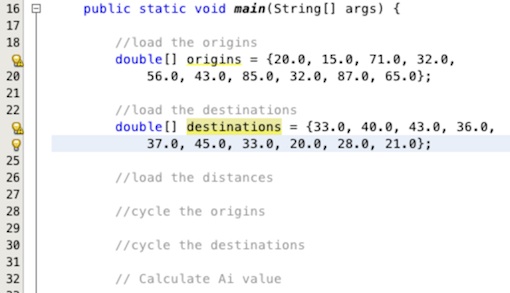
Now lets create the destination data. To do this we go through the same process. enter the line of code
double[] destinations = {33.0, 40.0, 43.0, 36.0, 37.0, 45.0, 33.0, 20.0, 28.0, 21.0}; into
the text editor area below our comment to get the destination data as shown in Figure 14.
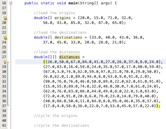
The last dataset we need to add in is the distances between the origins and destinations. This time
we are going to declare the array as a two dimensional array. The first dimension will represent the
origins and the second the destinations. To do this enter this line of code below the comment for loading
the distance data as demonstrated in Figure 15,
double[][] distances =
{{26.0,50.0,67.0,84.0,41.0,27.0,26.0,37.0,8.0,24.0},
{27.0,83.0,16.0,59.0,24.0,35.0,57.0,17.0,80.0,59.0},
{67.0,3.0,74.0,82.0,59.0,97.0,21.0,70.0,29.0,50.0},
{6.0,62.0,1.0,89.0,94.0,8.0,43.0,9.0,91.0,2.0},
{98.0,76.0,76.0,46.0,50.0,89.0,22.0,62.0,61.0,91.0},
{15.0,55.0,89.0,74.0,32.0,48.0,30.0,7.0,61.0,24.0},
{62.0,76.0,83.0,86.0,44.0,49.0,8.0,22.0,3.0,83.0},
{72.0,4.0,91.0,20.0,6.0,79.0,23.0,14.0,79.0,40.0},
{40.0,88.0,50.0,11.0,84.0,8.0,95.0,46.0,35.0,57.0},
{17.0,4.0,58.0,36.0,22.0,7.0,53.0,45.0,57.0,22.0}};
.
The distances is an array of arrays as explained in the arrays practical. Each set of braces
containing numbers represents an individual array. All of these arrays are included in another set of
outer braces which represents another array that holds all of the arrays defined within it. So a
to the two dimensional array of System.out.println(distances[2][5]); would print the value
at array element 2, which as we know would be the third array because out index starts at 0, and element 5
within that array which is?
Try find the answer manually yourself first and then you can try using the line of code above to print the value into the output window in Netbeans, don't forget to delete it again when done though! The answer you are looking for is below, so you can check that you have got it right.
answer = 97.0
Adding Loops:
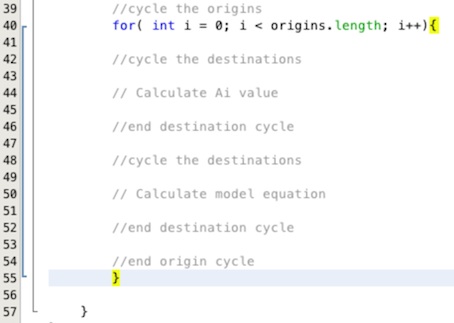
Now the data is in place we need to add the loops. The first loop is the outer origin loop. Add this
line of code in your text area under the comment for the origin loop as shown in Figure 16, for(
int i = 0; i < origins.length; i++){. Under the comment to close the origin loop add the closing
brace for the loop }.
Notice that we use i as the variable counter in the origin for-loop. This matches with the notation
used in the equations and is a general convention in social modelling theory.
In Figure 16 both the opening and closing brace for the loop are highlighted in yellow to help you locate the correct positions for them. Note, when you enter the first line of the for loop and press return, Netbeans will automatically be helpful and add the closing brace below. Please make sure that you either move this brace or delete it after adding your own in the correct location. If you don't your code will not compile.
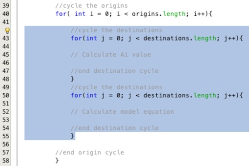
Now we can add the two destination loops around our two equations. Add this line below the two comments
for cycling the destinations, for(int j = 0; j < destinations.length; j++){. Add the closing
brace for each loop under the corresponding end of destinations cycle comment. Please remember to move or
remove any IDE automatically added braces. Your modified code should look like that in Figure 17.
Notice that we use j as the variable counter in the destination for-loops. This matches with
the notation used in the equations and is a general convention in social modelling theory.
Remember to tab your code in when inside the origins loop to nake it clear where our blocks start and end. To do this in one step highlight all of the code as it is in Figure 17, and press the tab key, to move it back out a step press shift and tab.
Insert the Equations:
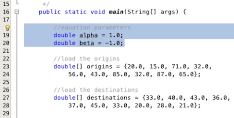
All that is left to do is enter the model equations. First of all we can add the calculation for the Ai values. To enable calibration of the model we insert parameters into the equations. These parameters are placed on the destination attractiveness and the calculation of distance. The parameters used in the literature are α and β. We will create two variables called alpha and beta.
Insert the following two lines of code before the data loading begins as shown in Figure 18,
double alpha = 1.0; and double beta = -1.0;.
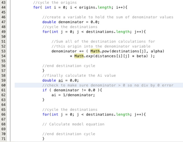
Now lets add the equation for calculating the Ai value for the current origin we are on in the loop.
- First we need a variable to add up the denominator for the Ai calculation as we cycle through the
destinations. Add this line of code above the start of the first destination for-loop,
double
denominator = 0.0;
. - Next we need to sum up all the values into the denominator. Add this line of code inside the loop,
remember to indent your code because you have now move inside another block,
denominator += (
Math.pow( destinations[j], alpha ) * Math.exp( distances[i][j] * beta ) );
. This line looks extremely complex but it is actually very simple. We raise the contents of the destination array at each element to the power of the value in α and multiply that by the exponential of the product of the distance between the current origin i and destination j. Each time we do this we add the new value to the existing values in our variabledenominatorusing the+=assignment command. There are a lot of brackets on this line to ensure the calculations are executed in the correct order. - Now we create a variable to hold the Ai value below the first destinations cycle. Insert this line
below the end brace for the first destinations cycle,
double ai = 0.0;. - Now we use another flow control statement to check and make sure that the value in the denominator is
not 0 and then we calculate ai. Below the variable you have just inserted add in the line
if ( denominator != 0.0 ){. This check if denominator does not equal,!=, 0. Below this and tabbed in again as we are inside another code block insert the actual calculationai = 1/denominator;and then immediately below this close the if block with a closing brace}.
That's it for the Ai value. Add some comments so that the code makes sense to you. You should end up with something similar to that in Figure 19.
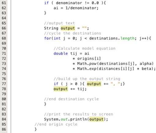
Now we can calculate the model equation. Insert this line into the second destination loop below the
calculate model equation comment, double tij = ai * origins[i] * Math.pow(destinations[j], alpha)
* Math.exp(distances[i][j] * beta);. All this line does is multiply each of the parts of the
equation together and store them in a new variable tij.
So that is the model done but we won't see any outputs, lets add a few lines to build up an output we can see.
- Above the second destination cycle loop create a string variable using this line of code
String
output = "";
. - Insert this line below the model equation calculation to add a comma before each value
for this origin except the first
if ( j > 0 ){ output += ", ";}. - Below this line add the flow value we have calculated to the output string,
output += tij;. - Finally, below the end of the second destinations loop but before the end of the origins loop add in
the line of code to output all of the flows from this origin to the screen,
System.out.println(output);.
That's it, add some comments to the code and you should end up with something like Figure 20 for the second destinations loop.
Run the code as you did at the beginning by right clicking on the SpatialInteractionModel.java file in the project area of the screen and selecting Run File. You should get an output like the one in Figure 21.
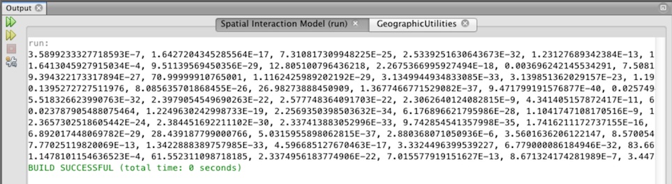
The output shows the flows from the origins going down the side to the destinations along the top. Try adjusting the α and β parameters to see what happens.
Summary
This practical has demonstrated how to build a basic origin constrained spatial interaction model using simple flow control statements and arrays. There are limitations, such as a lack of fitness measure and the absence of any calibration. The main points of the practical are:
- The Netbeans IDE groups code components together into projects.
- The IDE allows us to edit run and see output from our code all in one place.
- It is good practice to think about the implementation of your code and draw this up in comments before you start writing any code.
- Flow control statements such as for-loops and if statements allow us to branch and iterate within the code providing powerful processing tools.
- The Java programming language provides a wide variety of tools to make our lives easier, including common maths functions.