Multiscale Validation
In this part we'll use the software for validation.
We will take you through the task of validating some simulation results in the context of residential burglary.
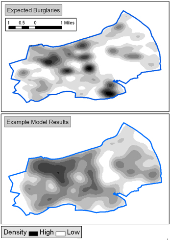
The simulated data are individual locations (points) of simulated burglaries and the observed (real) data are actual burglary locations around 2001 (we’ve randomised the locations slightly to anonymise the data). The figure to the right compares these two data sets visually by mapping the burglary density. Although there are clear differences between the simulated and real results, simply comparing data visually like this is not enough. We need a way to quantitatively compare the data.
The method that we use to validate the simulation here is called the "Expanding Cell" method which was developed by Andy and Nick (see Malleson et al. 2009) based on a method by Costanza (1989).
The method works by placing a square grid over the two point data sets and counting the number of points within each square. After this, it is possible to use traditional goodness-of-fit statistics such as the Standardised Root Mean Square Error (SRMSE) and R2 to quantitatively estimate the similarity of the two datasets (and hence the validity of the model). Also, the differences in counts in each cell can be mapped to show where the two datasets are similar and where they are different.
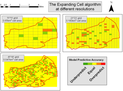
A nice feature of this type of approach is that it is possible to change the size of each square (and the number of cells in the grid), thereby comparing the datasets at a various spatial resolutions. For example, the figure to the right illustrates the similarity between two data sets using the expanding cell method at different resolutions.
We'll now run the test. Download and extract the following files somewhere convenient. They contain shapefiles (data mapable using ArcGIS) of east Leeds, Britain.
File 1: observed-adjusted.zip: the real (but slightly randomised) burglary data.
File 2: simulated.zip: the results of a model run to simulate burglaries.
Then run the software:
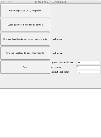
- Start the program (screenshot to the right).
- Tell the program were to find the expected and predicted data files.
- First click on Open expected (real) shapefile and navigate to the observed-adjusted.shp shapefile.
- Then click on Open predicted (model) shapefile and navigate to the simulated.shp file.
- Press Run! You don't need to change where the results are stored (by default all results are stored in the results directory).
The program works by first placing one large cell over the entire data set, then splitting this up into four smaller cells (2x2), then 9 (3x3) and so on. Each of these steps is called an iteration.
The "Upper limit" parameter determines the number of cells across the grid when the program should stop iterating and print the results (by default it will stops at 10, i.e. the last grid is 9x9). For each size, the grid is generated and error statistics calculated for each cell. The grid is then shifted 25% of the grid size in the four cardinal directions to generate 4 additional grid layers, each with its own calculations.
The "Output Grid Time" option says which layer-set of the size sequence to output as a map. All 5 shifted layers are output, with the statistics for the layers as cell attributes. If you set the Output Grid Time to "-1", you get the final, most detailed set of grids. Otherwise set it to the number of grid cells you want across the output map. The program also generates a CVS file containing the aggregate error statistics for each of the five grids for each size (it is interesting to see the variation in these, and how much effect grid shifting has).
The usual way of running an analysis is to generate the CVS, plot the change in error with grid size, and then use the "Output Grid Time" option to generate the 5 layers for a grid size of particular interest. These can be displayed simultaneously by setting the transparency of each to 20% in ArcGIS.
Having run the analysis now have a look in the results directory. There should be one file called results.csv and lots of shapefiles. Each of the shapefiles is a grid which is created after the program has finished.
Map the grids using ArcGIS to see where the model is similar to the expected data (use the "AbsPctError" field which shows the percentage difference between the counts in each cell; Right Click Shapefile layer in ArcMap --> Properties --> Symbology --> Quantities --> Graduated Colors – alter Value and Color Ramp).
If you map all the grids at once, change their transparency to 20%. Notice that on the whole the model and the real data are fairly similar, with the exception of a few small areas. If we wanted to calibrate the model now, we would try to work out why the results in these areas were worse than in others.
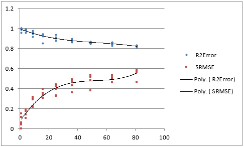
Finally look at the results.csv file and generate a graph which shows how the goodness-of-fit changes as the resolution of the grid increases (the cell size decreases). The graph should look something like that to the right.
On the graph we've stuck a 3rd order polynomial trend line. This helps us to think about questions such as "At what scale do we get the maximum fit to the real data, while keeping a good level of resolution". This might be dictated by the use of the model (if you are only interested in regional scale results, that's the scale to use, for example), but otherwise you might like to think about, for example, using the scale where the initial drop in error evens off, suggesting that the scale-correlation effects identified in the lecture are becoming less important and the spatial relationships between the observed and predicted points have been optimally overlapped. This may be the best scale at which you get a good predictability, but high detail.
References:
Costanza, R. (1989) Model goodness of fit: A multiple resolution procedure Ecological Modelling 47, 199-215.
Malleson, N.S., Heppenstall, A.J., See, L.M. and Evans, A.J (2009) Evaluating an Agent-Based Model of Burglary Working Paper 10/1, School of Geography, University of Leeds.