Agent Based Modelling: Introduction

Summary: Agent Based Modelling is, in some senses, the culmination of the methods we've looked at so far. It integrates crime and environmental data, along with behavioural and demographic data about offenders and victims to create a platform which can be used for both predictive estimation and theoretical studies.

Agent Based Models are computer models that attempt to capture the behaviour of individuals within an environment. They are more intuitive that mathematical or statistical models as the represent objects as we see them: as individual things in the world. The most familiar examples to many people will be The SIMs^™ or SIMCity^™ computer games in which people or other entities interact with each other and/or their environment. Because of the shift in computing languages over the last 30 years to Object Orientated Programming, which tries to deal with the world in much the same manner, ABMs have become reasonably simple to implement. In addition, their structure means that it is relatively simple to fold in a wide range of other techniques, including mathematical and statistical behavioural models.

Agent Based Models aim to provide a in silico lab, where we can:
1) Capture our understanding of systems.
2) Test that understanding of the systems for coherence and comprehensiveness.
3) See how theory at the individual level creates aggregate patterns.
4) Validate that theory against real data at the aggregate and individual scale.
5) Make predictions about the system.
6) Test "what if?" scenarios to inform planning

Background

Agent Based Models to some extent evolved from Cellular Automata (CA), and because of this, and because one of the first useful CA models (the Schelling model) was by a social scientist and has been re-implemented many times with ABM, it is worth saying something about CAs before we then go on to look at ABM.

CAs have been around since the earliest days of computing. They were first outlined by John Von Neumann in the 1950s, but took off in the 60s and 70s, especially after the publication by John Conway of the classic ruleset for emergence, The Game of Life. CAs are essentially a computer-created grid. Each cell in the grid has a set of possible states (for example, "alive" or "dead"). The model runs through a number of turns or "iterations". Each iteration, each cell in turn looks at the states of all the other cells within some immediate neighbourhood and sets its state based on those and its own current state. The complexity of the system comes from the rules used to convert the knowledge of states in the neighbourhood into the new state. As with any other complex system, simple rules can lead to very complex behaviour. Conway's Game of Life is a key example.

The CA grid can be one, two, or more dimensions. A classic one-dimensional CA is the model by Thomas Schelling (e.g. 1969), which he developed in the 1960s to look at ethic segregation in US cities. Schelling's model sets up a line of "0"s and "+"s to represent two ethnicities. He starts with them randomly spread along the line. He then gives them a 'mild' desire to live in neighbourhoods with people similar to themselves; let's say the cell under discussion is a "+", in this case they will tolerate 50&37; of people within 4 cells on either side of them being "0"s. If they find the "0"s in their neighbourhood are above that number, the cell is switched to a "0" and a "0" somewhere else changed to a "+" – the overall behaviour looks like the "+" has moved out of the neighbourhood to somewhere else. What Schelling found was that even with so-called 'mild' preferences, the line rapidly evolved to neighbourhoods of "+"s and neighbourhoods of "0"s. His argument was that out-and-out racism wasn't driving segregation, only a very mild preference (though, of course, now any preference would be counted as racism).

Schelling's model was done on paper initially, but it was rapidly converted to a CA, and soon after moved to two dimensions, where it displays considerable complexity. It still forms the core of many models that deal with movement and preference, and is still used in housing market models. One of the nice things about Schelling's model is it already points up many of the things we need to think about with both CAs and ABM: what the environment should look like; what rules we should give the people represented; what order should we update the people (if we always go left-to-right will that advantage some over others?); and when do we decide to stop the model?

Schelling's model actually sits on the CA-ABM continuum, as do many models. When Schelling first discussed the model he talked about people moving around the line. In general, one of the main distinctions between ABM and CAs is whether things move, or whether the just appear to because a series of cells change state. In an ABM objects in the world are represented as discrete entities, "agents", that know their location and actively move, carrying ancillary properties (like their name or age) with them. For example, if we look at this sequence:

00+0000
000+000
0000+00
00000+0

We might see this as the "+" moving right, but in a CA model it would be just a sequence of state changes in neighbouring cells. With an ABM the "+" would know where it was, and would shift that location from location = 3 to location = 4, 5, and 6. The key advantage is that the internal knowledge of the agent is maintained with the entity as it moves. With a CA, the movement of the "+" is only apparent – the knowledge associated with being a "+" does not travel with it.

Because agents carry knowledge with them as they move, they can utilise that knowledge and history as they travel around experiencing new areas and meeting other agents. Nevertheless, Markov systems (where behaviour in the next time step only depends on the current state) can be used to model a wide range of real-world systems, so CAs are still very popular. A classic example is the modelling of forest fires; whether a section of wood catches fire is largely determined by whether its neighbours are on fire and whether it is in an unburnt state.

Coding ABM

One of the nice things about ABM is how simple they are to start coding, and how far you can get with relative simplicity. Coding ABM is relatively simple because of the rise of Object Orientated Programming (OOP). OOP was a shift in the way programmes were written from the "shopping list" style of "proceedural programming" to one in which the code was divided into objects with a specific job to do, each object being based on a template called a "class" such that you can make multiple objects from each class definition and then change their internal states (which are usually multiple) to do different jobs. This maps clearly onto ABM, which, for example, our model defining a "Agent" class used to make multiple agents acting in different ways.

The classic ABM will therefore usually be based around the following:

An Agent class that contains variables associated with the agents and representing their states (name, age, location, etc. for a human) plus a chunk of code that can be run that enacts the behaviour of the agent. This chunk of code will be ring-fenced and called a name so it can be used, for example, most agents with variables containing their location would have a chunk of code called "move" that would move them when run. We call such chunks of code "procedures" or "methods".

A Model class that calls the agents' methods to get them to act. It is common to get agents to act a fixed number of times and then stop the model and look at the agents' states. Alternatively we may define a stopping condition and keep telling the agents to act until that is reached.

This is enough to build a simple agent based model where agents act based on their internal states, but at the moment they have nothing to interact with. Because of this, most ABM have some kind of environment all the agents know about; this may be as simple as a two dimensional array of data, or as complicated as a computer network. Each agent also tends to have a list of all the agents in the system so that it can interact with other agents, either all other agents, or just those whose location says they are close to the agent in question.

Below are some java files that build up a very simple ABM of crime. They form a "cops and robbers" model, in which robbers randomly wander around a space looking for banks to rob, but also rob each other, and where cops wander round randomly taking the gold off robbers and removing them from the model / arresting them. You don't need to understand the detail of the java if you're not a programmer, but it is worth having a look at 1) to show you that there's not a lot of code involved; 2) to give you some idea of how these models are constructed; and 3) to give you the chance to think through how you could start to adapt this behaviour to build more realistic models.

Agent.java
Model.java

If you want to run this model, download this zip file: model.zip, unzip it into a directory somewhere and go to that directory in Windows Explorer / Mac Finder. In Windows, right-click on an empty space in the directory while holding the SHIFT key, and select "Open Command Window" or similar from the menu. Once you have this "command prompt" or "terminal" open, type in the following and push Enter to run the model:

java Model

In the event that it doesn't work, you may need to download the latest Java Runtime. If it does work, you can adjust the number of agents, the number of iterations, and the probability that an agent is a cop by giving the following command line attributes, thus:

java Model numberOfAgents(whole number) iterations(whole number) probabilityOfCop(between 0 and < 1)

e.g.

java Model 100 200 0.2

This may not seem very sophisticated, and, indeed, it isn't. However, it is a basic ABM. A sophisticated ABM would probably have a stronger set of decision making rules about who and when to rob someone, for example. Indeed, a lot of ABM have formal cognitive models that decision making is embedded within. The classic example of the is the Belief-Desire-Intention (BDI) model. This centres decision making around variables and behaviours that represent Beliefs – facts about the world which can be rules; Desires – things the agent wants to do / make happen; and Intentions – actions the agent has chosen, usually from a set of plans. For a good introduction to the BDI structure, see Wooldridge (2009), which is a good introductory text on a range of issues in ABM.

BDI decisions are usually made by assuming a utility function. This might include:
1) whichever desire is most important wins;
2) whichever plan achieves most desires;
3) whichever plan is most likely to succeed;
4) whichever plan does the above, after testing in multiple situations;
5) whichever a community of agents decide on (eg by voting).

So you can see that the sophistication of the decision making can be much more involved. It's also worth saying that you are not limited to the kind of if-this-variable-do-this rules in the model above; rules can be mathematical, statistical, logical, or linguistic, for example. One of the strengths of ABM is that it is simple to integrate a wide variety of methodology from other modelling areas.

Issues in ABM

As we saw with the Schelling example, there are a large number of things to consider when building an ABM. These include:

Whether to make it an abstract model of a system, or based on real world detail.
How to make sure you have the computing memory and power to run the model.
What order to run the agents in, and how to set them running.
How to pick parameters values for the variables that determine their actions.
How to tell when the model has 'worked'

We'll look at some of these issues now.

Abstract vs Realism

Broadly speaking, most modellers fall into two camps: those who think you can never model the real world in detail, and think that you should treat models as elaborate thought-experiments, vs those who think it is possible to build detailed models of the real world and make predictions on that basis. This leads to two style of model. The first is abstract models which concentrate on a limited set of processes, initialised often with educated guesses, and which are chiefly used by manipulating elements to explore system responses. The second is the 'kitchen-sink' model, which has as much as possible of the real world represented inside it, with the system initialised by real world data. As these models are often initialised with real data, use real data in calibration (see below) and validation (see below), they are very data-reliant. Fortunately (or unfortunately) in crime studies this is less of an issue that it might be in over areas.

As real systems are rarely discrete from the rest of reality, there's no real answer to which of these types of model is better, and, indeed, they both have their uses. Pragmatically, the abstract models are often easier to build, as the generally rely on literature and the modeller's intuition, while the more detailed models require large amounts of real-world data and include more processes. However, the potential usefulness for practitioners of the more complicated models rewards their investment. Overall, however, the distinction is, to a degree, fallacious: both sets of models are founded on knowledge from the real world, both give artificial closure to systems that aren't closed, both can be used predictively, but also both act as a medium where one can store knowledge and test it for consistency in a complicated set of interlinked processes.

One of the most immediate ways in which the level of realism plays out is in the space that agents inhabit. These can be a wide range of types and level of detail. Which you pick will depend on the level of realism and data use you need.

Boundary types are important; what happens at the edges of worlds? Choices include:
1) Pseudo-Infinite plains
2) Bound areas where data outside the margin is forbidden
3) Bound areas where data outside the margin is accessible, but agents can't leave
4) Torus geometries (where leaving one side brings you back on the other)

The organisation of space also varies; space can be:
1) Continuous
2) Gridded (square; triangular; hexagonal; other)
3) Irregular areas, or quad-trees
4) Networks

In addition, the neighbourhoods within which agents can see each other can vary, in part depending on the spatial organisation. They can be:
1) Moore neighbourhoods (square on a grid)
2) Von Neumann (diamond on a grid)
3) Diagonal on a grid
4) Euclidian in continuous space
5) Network distances

Memory and Power

One of the chief issues with trying to build a model of individual objects in the real world is that it takes a great deal of computer memory to do it, and a great deal of computing power to run through each object getting it to act. Things have improved a lot in this regard, but of course as resources have improved, our desire to build bigger models, especially founded on so-called "Big Data" have expanded. Agent Based Models of the global population are certainly within our capacity, but making them detailed requires huge resources.

It is instructive to think about the levels of computer memory needed (and here we mean quickly accessible memory for processing, that is RAM, rather than harddrive memory). If we want to store a geographical location we may need the computer to set aside space for an integer number for the degree, another for the minutes, another for the seconds, and another for the sub-seconds. In addition, we'll need these for both longitude and latitude: eight numbers in total. Computer memory is allocated in small spaces called 'bits', and storing eight numbers could take some 256 bits. This means that in 1Gigabyte of memory space we could store the location of 33,554,432 people. This isn't including: 1) the fact that we're likely to need multiple values per person; 2) that we need to store the running code. Infact, these storage issues mean we're only ever likely to get between 100,000 and 1,000,000 agents on a single PC, and for agents with very complicated cognitive models, this may drop to one or two agents.

Equally, processing time becomes important. Take two models we've worked on:
a) Individual level model of 273 burglars searching 30000 houses in Leeds over 30 days takes 20hrs (Malleson, 2010).
b) Aphid migration model of 750,000 aphids takes 12 days to run them out of a 100m field (Parry and Evans, 2008).

These times don't seem so bad, however, as we'll see shortly, we usually want to run models hundreds of times. Even if we only run these models a hundred times, we get:
a) 100 runs of the burglary model takes 83.3 days
b) 100 runs of the aphid model takes 3.2 years

While it wouldn't be out of the question to run a model for a month, when we get to these scales, special resources are needed. So, what are the solutions? If a single model takes 20hrs to run and we need to run 100:
a) Batch distribution: Run models on 100 computers, one model per computer. Each model takes 20hrs. Only suitable where not memory limited.
b) Parallelisation: Spread the model across multiple computers so it only takes 12mins to run, and run it 100 times. Here we divide up agents, data, of some of the jobs the model does between different machines and link everything together at intervals.
c) Somehow cut down the number of runs needed.

(a) is undoubtedly easiest, however if our model is memory-limited we'll have to divide the memory-heavy components using (b), even though this means communicating between multiple computers, which usually slows down run-times. Sometimes it is better to get a model running slowly than not at all. If we do decide we need to parallelise our model, we then need to decide how to divide it up. One option is to divide up the agents and the geography associated with them - simple to do if the agents are static and don't talk to each other much as it means separate machines can deal with groups of agents acting on a subset of the data. If agents move a lot, but don't talk to each other, you can give each machine a copy of the whole environment and let sub-sets of the agents wander about on each machine. Unfortunately, most models have agents that move and communicate so at some point you have agents trying to move to, or talk to agents on, other machines, and this brings a network communication overhead between the machines. For some ideas about dealing with this issue, see Parry and Evans (2008).

Timing and synchronisation

One issue with agents is when you ask them to run their code. There are broadly two options: in the first, agents are called after a specific number of clock intervals, often called "ticks". Quite often agents are called every tick, and ticks then represent some fundamental timescale, usually dictated by the data the model is using (if collected yearly, hourly, etc.). The second option is called "event based" activity, and with this way of working agents are individually asked to run their code when something significant to them happens (for example, another agent gets in touch). The tick model is much simpler to implement, but may be less effective where large numbers of agents are inactive each round, or where behavioural realism is needed. In general, even with an event based system, there will be a system clock that agents can refer to if they want to synchronise actions with other agents.

Where agents all act to a clock, an additional issue arises, which is the order in which agents are called. Calling the agents in the same order all the time can cause model artefacts, that is, patterns that are due to the model and wouldn't appear in the real world. For example, if an agent always moves first, it may gain an advantage over other agents it wouldn't have in the more random real world. For this reason it is usual to randomise the order agents are run each time.

Calibration

Any model, however behaviour based, will sooner or later need some values inside it to adjust behaviours or cope with a lack of system knowledge about the real world – for example, if our agents are going to see other agents, how far can they see? If you need to pick such "parameters", we need to decide how this will be done so the model best matches reality. If we're not sure what the values might be, this process of picking values is known as "calibration". We have various options:
1) Using expert knowledge. This can be helpful, but experts often don't understand the inter-relationships between variables as well as they might.
2) Experimenting is lots of different values. This is rarely possible with more than two or three variables because of the combinatoric solution space that must be explored.
3) Deriving them from data automatically using AI/Alife techniques. This is a large area, but one of the most commonly used. A typical example is to use a Genetic Algorithm.

Validation

Proving the model 'works' depends on identifying first what we mean by 'working'. In general models are validated against real world patterns. For abstract models this is usually about replicating behaviours, while for more 'realistic' models, this involves checking values and locations against real data. If this is the comparison we need to make, we then need to decide how that comparison will proceed. Options include:
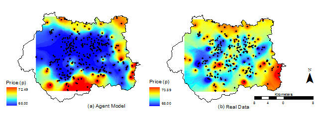
Visual or "face" validation: e.g. Comparing two city forms.
One-number statistic: eg. Can you replicate average price?
Spatial, temporal, or interaction match: e.g. Can you model city growth block-by-block?

The simplest example of a one-number, global, statistic we might use is the Total Absolute Error (TAE). If we're just predicting continuous values, we take values in one dataset from another, and sum the absolute differences.

For categorical data, for example if we're predicting urban vs rural areas, we can construct a confusion matrix / contingency table: for each predicted area, what category is it in really, and in the prediction.

Example contingency table

	Predicted A	Predicted B
Real A	10 areas	5 areas
Real B	15 areas	20 areas

We can then use these to generate a statistical representation of the mismatch in categories per area, such as the Kappa statistic (e.g. Sousa et al., 2002).

These kind of statistics are ok, but don't do so well where we're making categorical predictions in space. This is because we may be out in either space (predicting the right category, but in slightly the wrong place), or category (right place, but wrong category), or both.

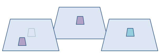
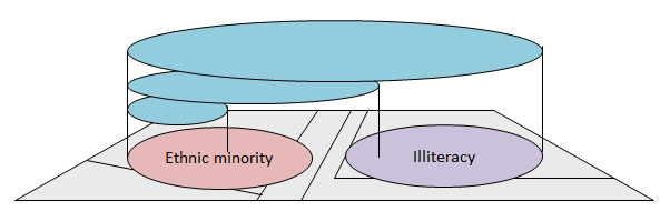
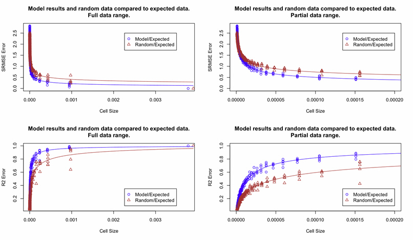
The solution is a fuzzy category statistic and/or multiscale examination of the differences (see, for example, Costanza, 1989). With a multiscale statistic we scan across the real and predicted map with a larger and larger window, recalculating the statistics at each scale. At this stage we might imagine that we look for the scale at which we have the strongest correlation between them – this will be the best scale the model predicts at? The trouble is, scaling up and calculating correlation statistics up will always increase correlation coefficients. Correlation coefficients tend to increase with the scale of aggregations. Robinson (1950) compared illiteracy in those defined as in ethnic minorities in the US census and found high correlation in large geographical zones, less at state level, but none at individual level. Ethnic minorities lived in high illiteracy areas, but weren’t necessarily illiterate themselves. As areas of effect overlap more and more, the correlation rises:

We therefore need to look carefully at scaling statistics and look for points where the maximum gain in predictability is traded off well against the smallness of scale. This will give us the most practical scale of prediction.

Of course, an exact prediction is unlikely, and, actually, quite often we may be interested in where models fails rather than how it doesn't. If models represent our current understanding, failure may reveal important dynamics we haven't recognised. Nevertheless, if we do want a perfect match and don't get it, how can we assess how good a job we've done. Statistics like the TAE give us how close we are, but they don't include any notion of what that means. These kind of statistics are good if we want to get closer and closer to a realistic prediction (for example, if we're assessing calibrations), but they don't tell us how 'well' we've done if we don't get an exact prediction.

One option is to randomisation the elements of the prediction; eg. can we do better at geographical prediction of urban areas than randomly throwing them at a map? Or, alternatively, how likely is it we'd see this pattern if the process was random? The trouble is, this doesn't always seem a fair comparison; after all, models will often be initialised with real data with a pattern already inherent in it. An alternative is the "Business-as-usual" model; if we can’t do better than just keeping the a past situation and treating that as an alternative prediction, we’re not doing very well. However, this assumes no known growth, which the model may not – that is, models may be forced to change where no change is better. Overall, decisions as to how 'well' a prediction is doing can be problematic and it is simpler to pragmatically say "model A does better that model B", or "this model makes a prediction with this level of error at this scale".

Errors

Model errors will come from a number of sources. There will be errors associated with the input data, errors associated with the model parameters being incorrect, and errors associated with the model structure (amungst others: see Evans, 2012 for a review and discussion of solutions). We need to be able to assess the variation of the model associated with these errors so we can determine how closely a model is likely to ever match reality.

One technique is "sensitivity testing"; we slightly vary key variables to see how the model responds at output. This is one of the reasons we might want to run hundreds of model runs. The model maybe ergodic, that is, insensitive to starting conditions after a long enough run, or it may be very sensitive. If the model does respond strongly is this how the real system might respond, or is it a model artefact? If it responds strongly what does this say about the potential errors that might creep into predictions if your initial data isn't perfectly accurate? We need to decide whether error propagation through the system, especially where an error magnifies repeatedly, is a problem. Plainly an unstable model of a stable system is problematic. Many people think this is a major issue with ABM – that nonlinearities in the models destroy any attempt to use the predictively. However, we have to ask what it is in the real system that usually stabilises it, that is, what are the homeostatic processes? These are often the elements that are missing from models. Processes like agent-to-agent negotiation, averaging, and aggregation will often dampen down error propagation.

Frequently the input data for repeated model runs will be sampled probabilisticly from collections of input data so that the inputs have the distribution of real data, but without repetition – so-called Monte Carlo sampling. This not only reduces the change of harmonics developing in the model because we've fed the same data in multiple times, but also gives the opportunity for building up a large collection of probabalistic results rather than a single output for a single input dataset. Again, to do this we may have to run hundreds of model runs. However, this Monte Carlo testing is key to exploring the error and uncertainty associated with input data, as well as assessing how parameter variation affects models.

Summary

In total, these sections have tried to sum up some of the difficulties associated with ABM, and some of the considerations we need to make. While some of these issues may seem very problematic they are by no means fatally so. The key is often to start with a simple abstract model that captures understanding of a system. Just being able to store knowledge and look at the conflicts between our understandings, and how our understanding of individuals plays at a larger scale is a major advance. Additional work to build on that foundation is then solidly based, and repays whatever effort can be made to work with some of the issues above.

Useful courses

Volker Grimm and Steve Railsback (see reading, below), run two extremely well respected courses in ABM modelling with NetLogo. You can find out more on their book website.

For those wanting to learn how to code ABM from scratch, Andy Evans ran an annual course teaching Java programming using building up an ABM as the example. You can find all the course materials, recorded lectures, code, etc. online and free to use.

References

Wooldridge, M. (2009) An Introduction to MultiAgent Systems Wiley (2nd Edition).

Railsback, S.F. and V.Grimm (2011) Agent-Based and Individual-Based Modeling: A Practical Introduction Princeton University Press.

Russell, S. and P. Norvig (2010) Artificial Intelligence: A Modern Approach Prentice Hall (3rd Edition)

References

Constanza, R., (1989) Model goodness of fit: a multiple resolution procedure. Ecological Modelling 47, 199-215

Evans, A.J. (2012) Uncertainty and Error. In Heppenstall, A.J., Crooks, A.T., See, L.M., and Batty, M. Agent-Based Models of Geographical Systems. Springer.

Gehlke, C.E. and Biehl, H. (1934) Certain effects of grouping upon the size of correlation coefficients in census tract material Journal of the American Statistical Association, 29 Supplement, 169-170.

Hagen-Zanker, A.  (2009) An improved Fuzzy Kappa statistic that accounts for spatial autocorrelation. International Journal of Geographical Information Science, 23 (1), 61-73  

Heppenstall, A.J., Evans, A.J. and Birkin, M.H. (2005) A Hybrid Multi-Agent/Spatial Interaction Model System for Petrol Price Setting. Transactions in GIS, 9 (1), 35-51

Malleson, N. (2010) Agent-Based Modelling of Crime. unpublished PhD, University of Leeds.

Malleson, N., See, L.M., Evans, A.J. and Heppenstall, A.J. (2010) Implementing comprehensive offender behaviour in a realistic agent-based model of burglary. Simulation, 0(0): 1-22

Monserud, R.A. and R. Leemans (1992) Comparing global vegetation maps with the Kappa statistic. Ecological Modelling, 62 (4), 275-293

Parry, H., Evans, A.J., and Morgan, D. (2006) Aphid population dynamics in agricultural landscapes: an agent-based simulation model. Ecological Modelling, Special Issue on Pattern and Processes of Dynamic Landscapes, 199 (4), 451-463.

Parry, H. and Evans, A.J. (2008) A comparative analysis of parallel processing and super-individual methods for improving the computational performance of a large individual-based model Ecological Modelling, 214 (2-4), 141-152

Railsback, S.F. and V.Grimm (2011) Agent-Based and Individual-Based Modeling: A Practical Introduction Princeton University Press.

Robinson, W.S. (1950) Ecological correlations and the behaviour of individuals. American Sociological Review, 15, 351-357.

Schelling, T.C. (1969) Models of Segregation in: Strategic Theory and Its Applications, Schelling, T.C. The American Economic Review, 59 (2), Papers and Proceedings of the Eighty-first Annual Meeting of the American Economic Association. (May, 1969), pp. 488-493.

Sousa, S., S. Caeiro and M. Painho, (2002) Assessment of Map Similarity of Categorical Maps Using Kappa Statistics, ISEGI, Lisbon.

Thiele, J.C., W. Kurth and V. Grimm (2104) Facilitating Parameter Estimation and Sensitivity Analysis of Agent-Based Models: A Cookbook Using NetLogo and R. Journal of Artificial Societies and Social Simulation 17 (3) 11