Spatial microsimulation

Summary: Spatial microsimulation is a technique for estimating the characteristics of a population. It allows us to combine traditional census-style aggregate statistics about an area with smaller scale and more specific surveys to generate a population that contains estimated characteristics from both. As such it is a useful technique for estimating populations at risk from crime and levels of, for example, fear of crime.

Spatial microsimulation is a technique that estimates what individuals are like in an area, based on aggregate statistics. In its simplest form it just generates a set of individuals, the characteristics of which match aggregate statistics for an area. For example, say we knew the aggregate levels of employment and income in an area, and wanted to allocate employment and income to individual houses in that area, simple spatial microsimulation would generate synthetic individuals that we could allocate to houses, whose employment and income, when aggregated would give us the area statistics.

However, in addition, spatial microsimulation can be used to estimate the levels of additional variables, so if we know there is a strong national-level relationship between income, employment, and fear of crime, we can generate the level of fear of crime in our synthetic individuals. In general, because of the relationships between the constraints used, the technique usually does better than a multivariant regression.

Microsimulation comes in a wide variety of forms, and spatial microsimulation specifically has a number of variants. However, the overall idea with spatial microsimulation is to generate an individual-level population that is a good estimate of people in an area. The usual reason for having to do this is because census microdata is protected. However, spatial microsimulation can also be used to estimate the distribution of characteristics for an area that are unavailable for that area in an aggregate form.

The simplest version of spatial microsimulation takes two datasets: statistics about an area, say aggregate census statistics, and a sample of individuals, say an anonymised sample of the census microdata, and uses the latter to construct a population that matches the former. Note that the sample of individuals does not have to be drawn from the area in question (indeed, usually isn't) as long as it is likely that at least some of the people in the sample are similar to the kinds of people that might be in the area.

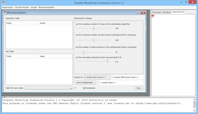
The algorithm we'll look at for constructing this population starts by randomly sampling the sample and placing people in the area until the correct number of people is built up. Obviously at this point the characteristics of the people won't match the aggregate statistics, other than in total population numbers. If we choose a set of variables we're interested in we can build up an error statistic between the aggregate statistic we'd like to generate and the current aggregate statistic generated from the randomised population. We might pick, say, five variables to do this for; these are our constraints – the variables we'd like to match. At its heart, algorithm then involves swaping people out of the population for others from the sample of individuals and seeing if the swap improves the error statistic. If it does, we keep the swap, if it doesn't, we reverse it, and swap again with someone different. Those familiar with optimisation might recognise this as a Greedy Algorithm, and like other uses of this algorithm there are more complicated meta-heuristic algorithms we can impose on top of this to make it more effective. For example, Kirk Harland's microsimulation toolkit built into the free, open source, FMF utilises Simulated Annealing (this is currently the only out-of-the-box software to do spatial microsimulation).

Eventually, if we continue this swapping, the synthetic population will converge on the statistics associated with the real population. How close it gets depends on the breadth of people in the sample and the number of constraining variables used. Matching a single variable, like sex, is trivial, but when there are seven or eight variables to match against, swapping in an individual will often improve the score for one variable but make another worse, and there may be no individual in the sample that will match the deficit. The meta-heuristic algorithms help with this, in that they generally allow some backtracking or low-level temporary error acceptance, but there may, at the end of the day, be no perfect solution. Nevertheless, the algorithm does a pretty good job in most circumstances.

This simple algorithm hides one additional advantage the method has, which is to estimate population characteristics that are not in the aggregate statistics, but are in the sample of individuals. While we may quite often use aggregate statistics and a sample of individuals drawn from the same survey (e.g. a census), we may instead use different surveys where the constraining variables used link the two datasets, but where the sample of individuals otherwise contains very different data (for example, a crime survey that contains the demographic variables of the census, but also variables on victimisation and fear of crime). Dragging an individual into the synthetic population will also drag variables into the population that aren't the constraining variables. Provided there is a correlation between the characteristics an individual in the sample has, these ancillary variables will then be an estimate of the ancillary variable levels in the population. Obviously the stronger the correlation with other characteristics, the better this estimation will be. At worst, if the ancillary variables are independently correlated with one or more of the constraining variables, this method will do as well as standard regression, but where there is a non-linear relationship between all the variables it is likely to do better.

Finally, one can distinguish between static microsimulation, of the type discussed here, and dynamic microsimulation, which then takes the populations generated and rolls them forward using probabalistic functions – for example, a birth and death rate. The distinction is somewhat confused by the fact that the algorithm we've described is sometimes called dynamic optimisation microsimulation, despite the result being a static symulated population. As well as dynamic roll-forwards, microsimulated populations can act as the foundation for an Agent Based Model that adds interaction between the individuals, and the individuals and the environment they live in.

Once you're ready, you use the Flexible Modelling Framework to run your own microsimulation.

Useful reading

Dimitris Ballas’ free online book summarises the Dynamic Optimisation methodology used in the Flexible Modelling Framework Microsimulation plugin, and discusses some of the issues. It also lists some useful microdata datasets:
Ballas, D., Rossiter, D., Thomas, B., Clarke, G.P. and Dorling, D. (2005). Geography matters: simulating the local impacts of national social policies. Joseph Rowntree Foundation contemporary research issues, Joseph Rowntree Foundation, York. ISBN 1859352650.

There is an alternative microsimulation technique which gets to the same point via a different route, called Iterative Proportional Fitting. This can generate a better fit if you have smaller microdata samples, but doesn’t generate whole individuals. You can find out more about this in Robin Lovelace’s free online book, which is currently under development, but is in an almost final form:
Lovelace, R. (in prep) Spatial Microsimulation with R. CRC Press.

Finally, for an academic overview of some of the techniques and their issues, see:
Harland, K., Heppenstall, A.J., Smith, D. And Birkin, M. (2012) Creating realistic synthetic populations at varying spatial scales: A comparative critique of population synthesis techniques. JASSS. 15(1) 1.